Skip to main content

Turning documents into categories

Follow the text-classification recipe on inaugural paragraphs

Learn how a text classifier represents documents, fits a model, returns probabilities, and needs a cut point.

Elena has a box of labelled speeches and a simple question for the archive search page. Could a paragraph’s vocabulary help sort it into a broad time period?

The page must be careful. A classifier can find differences in wording without explaining history, policy, or people. This lesson treats the inaugural corpus as a technical corpus for vocabulary practice and nothing more.

TipWhat you will learn

By the end of this lesson, you will be able to:

• name the four steps in a text-classification recipe;
• compare token counts with term frequency-inverse document frequency;
• read a baseline beside a model score;
• inspect a probability distribution; and
• explain why a cut point is a separate choice.

Load the shared corpus

The inaugural addresses come bundled with quanteda and are works of the United States government. The shared helper creates 1,377 paragraphs from 60 speeches. readr opens the committed score files, dplyr and tibble shape tables, ggplot2 draws the probability chart, and tidymodels with textrecipes and glmnet fits the models.

library(readr)
library(dplyr)
library(tibble)
library(tidyr)
library(purrr)
library(stringr)
library(ggplot2)
library(tidymodels)
library(textrecipes)
library(glmnet)
library(quanteda)

source("R/inaugural-corpus.R")
paragraphs <- inaugural_paragraphs()

split_study <- read_csv(
  "data/inaugural/split-study.csv",
  na = "NA",
  col_types = cols(
    task = col_character(),
    split_scheme = col_character(),
    replicate = col_integer(),
    accuracy = col_double(),
    bal_accuracy = col_double(),
    train_majority_accuracy = col_double(),
    test_majority_rate = col_double(),
    length_rule_accuracy = col_double(),
    test_rows = col_integer(),
    test_speeches = col_integer()
  )
)

baselines <- read_csv(
  "data/inaugural/baselines.csv",
  na = character(),
  col_types = cols(
    task = col_character(),
    outcome = col_character(),
    rows = col_integer(),
    speeches = col_integer(),
    people = col_integer(),
    largest_class = col_character(),
    baseline_accuracy = col_double()
  )
)

era_counts <- paragraphs |>
  count(era, name = "paragraphs")

era_evidence <- split_study |>
  filter(task == "era", split_scheme == "speech") |>
  summarise(
    speech_split_accuracy = mean(accuracy),
    split_minimum = min(accuracy),
    split_maximum = max(accuracy),
    split_spread = split_maximum - split_minimum,
    deployable_baseline = mean(train_majority_accuracy),
    length_rule_accuracy = mean(length_rule_accuracy),
    replicates = n(),
    .groups = "drop"
  )

era_baseline_metadata <- baselines |>
  filter(task == "era")

knitr::kable(
  era_counts,
  col.names = c("Era label", "Paragraphs"),
  caption = "Paragraph labels created by the shared inaugural helper",
  row.names = FALSE
)

Paragraph labels created by the shared inaugural helper

Era label	Paragraphs
before 1900	485
1900 or later	892

knitr::kable(
  era_evidence |>
    mutate(across(where(is.double), \(value) round(value, 4))),
  col.names = c(
    "Mean speech-level accuracy",
    "Minimum replicate",
    "Maximum replicate",
    "Replicate spread",
    "Train-majority baseline",
    "Paragraph-length rule",
    "Replicates"
  ),
  caption = "Committed evidence for the era classifier",
  row.names = FALSE
)

Committed evidence for the era classifier

Mean speech-level accuracy	Minimum replicate	Maximum replicate	Replicate spread	Train-majority baseline	Paragraph-length rule	Replicates
0.8457	0.797	0.9039	0.1069	0.6282	0.6827	10

The committed study reports 0.8457 mean accuracy across 10 speech-level splits. Those 10 replicate scores run from 0.7970 to 0.9039, so a single split can land above or below the mean. The deployable train-majority baseline averages 0.6282: it chooses the majority label from the training split, then applies that choice to the test split. A paragraph-length-only rule averages 0.6827. The corpus has 60 speeches by 40 people. Lesson 44 covers evaluation methodology; this page focuses on how representation changes the model’s input.

Those committed numbers come from ridge models with stop-word removal and unstratified speech-grouped splits. The live comparison below uses lasso models, keeps stop words, and stratifies its speech splits. Read the committed table as context for the task, not as a score comparison with the live fits.

Represent the text

Text classification follows four steps: represent the text, fit a model, predict a score, then decide what score becomes a label. A feature is an input column for the model. Here the features are words after tokenization.

Two common representations are token counts and term frequency-inverse document frequency, often shortened to tf-idf. A count records how often a word appears. tf-idf gives less weight to words that appear in many documents.

set.seed(5101)
speech_split <- group_initial_split(
  paragraphs,
  group = speech_id,
  prop = 0.75,
  strata = era
)
era_train <- training(speech_split)
era_test <- testing(speech_split)

fit_era_model <- function(use_tfidf = TRUE, max_tokens = 500L) {
  model_recipe <- recipe(era ~ paragraph, data = era_train) |>
    step_tokenize(paragraph) |>
    step_tokenfilter(paragraph, max_tokens = max_tokens)

  if (use_tfidf) {
    model_recipe <- model_recipe |>
      step_tfidf(paragraph)
  } else {
    model_recipe <- model_recipe |>
      step_tf(paragraph)
  }

  workflow() |>
    add_recipe(model_recipe) |>
    add_model(
      logistic_reg(penalty = 0.01, mixture = 1) |>
        set_engine("glmnet") |>
        set_mode("classification")
    ) |>
    fit(data = era_train)
}

set.seed(5102)
era_tfidf_fit <- fit_era_model(use_tfidf = TRUE, max_tokens = 500L)

set.seed(5103)
era_count_fit <- fit_era_model(use_tfidf = FALSE, max_tokens = 500L)

score_era_model <- function(fitted_workflow) {
  probability_table <- predict(fitted_workflow, era_test, type = "prob")
  late_column <- names(probability_table)[str_detect(names(probability_table), "later")]

  era_test |>
    select(paragraph_id, era) |>
    bind_cols(probability_table, predict(fitted_workflow, era_test)) |>
    mutate(prob_1900_or_later = .data[[late_column]])
}

tfidf_scores <- score_era_model(era_tfidf_fit)
count_scores <- score_era_model(era_count_fit)

feature_comparison <- tibble(
  representation = c("tf-idf, 500 tokens", "token counts, 500 tokens"),
  accuracy = c(
    yardstick::accuracy(tfidf_scores, truth = era, estimate = .pred_class) |>
      pull(.estimate),
    yardstick::accuracy(count_scores, truth = era, estimate = .pred_class) |>
      pull(.estimate)
  )
)

feature_gap <- abs(diff(feature_comparison$accuracy))

score_feature_split <- function(split_seed) {
  set.seed(split_seed)
  replicate_split <- group_initial_split(
    paragraphs,
    group = speech_id,
    prop = 0.75,
    strata = era
  )
  replicate_train <- training(replicate_split)
  replicate_test <- testing(replicate_split)

  fit_replicate_model <- function(use_tfidf, fit_seed) {
    replicate_recipe <- recipe(era ~ paragraph, data = replicate_train) |>
      step_tokenize(paragraph) |>
      step_tokenfilter(paragraph, max_tokens = 500)

    if (use_tfidf) {
      replicate_recipe <- replicate_recipe |>
        step_tfidf(paragraph)
    } else {
      replicate_recipe <- replicate_recipe |>
        step_tf(paragraph)
    }

    set.seed(fit_seed)
    workflow() |>
      add_recipe(replicate_recipe) |>
      add_model(
        logistic_reg(penalty = 0.01, mixture = 1) |>
          set_engine("glmnet") |>
          set_mode("classification")
      ) |>
      fit(data = replicate_train)
  }

  tfidf_fit <- fit_replicate_model(use_tfidf = TRUE, fit_seed = split_seed + 1000L)
  count_fit <- fit_replicate_model(use_tfidf = FALSE, fit_seed = split_seed + 2000L)

  bind_rows(
    tibble(
      representation = "tf-idf, 500 tokens",
      accuracy = yardstick::accuracy(
        bind_cols(replicate_test |> select(era), predict(tfidf_fit, replicate_test)),
        truth = era,
        estimate = .pred_class
      ) |>
        pull(.estimate)
    ),
    tibble(
      representation = "token counts, 500 tokens",
      accuracy = yardstick::accuracy(
        bind_cols(replicate_test |> select(era), predict(count_fit, replicate_test)),
        truth = era,
        estimate = .pred_class
      ) |>
        pull(.estimate)
    )
  ) |>
    mutate(split_seed = split_seed, test_rows = nrow(replicate_test))
}

feature_replicates <- bind_rows(
  feature_comparison |>
    mutate(split_seed = 5101L, test_rows = nrow(era_test)),
  map(5102:5105, score_feature_split) |>
    list_rbind()
) |>
  relocate(split_seed)

feature_summary <- feature_replicates |>
  summarise(
    mean_accuracy = mean(accuracy),
    minimum = min(accuracy),
    maximum = max(accuracy),
    spread = maximum - minimum,
    .by = representation
  )

feature_gaps <- feature_replicates |>
  select(split_seed, representation, accuracy) |>
  pivot_wider(names_from = representation, values_from = accuracy) |>
  mutate(gap = abs(`token counts, 500 tokens` - `tf-idf, 500 tokens`))

test_counts <- era_test |>
  count(era, name = "paragraphs")

knitr::kable(
  feature_comparison |>
    mutate(accuracy = round(accuracy, 4)),
  col.names = c("Representation", "Accuracy on this split"),
  caption = "Changing features changes the result on the same speech-level split",
  row.names = FALSE
)

Changing features changes the result on the same speech-level split

Representation	Accuracy on this split
tf-idf, 500 tokens	0.8799
token counts, 500 tokens	0.8949

knitr::kable(
  feature_summary |>
    mutate(across(c(mean_accuracy, minimum, maximum, spread), \(value) round(value, 4))),
  col.names = c("Representation", "Mean accuracy", "Minimum", "Maximum", "Spread"),
  caption = "Five same-configuration speech-level splits for each representation",
  row.names = FALSE
)

Five same-configuration speech-level splits for each representation

Representation	Mean accuracy	Minimum	Maximum	Spread
tf-idf, 500 tokens	0.8381	0.7632	0.8799	0.1167
token counts, 500 tokens	0.8477	0.7690	0.8966	0.1275

On this split, token counts score 0.8949 and tf-idf scores 0.8799. The gap is 0.0150. With the same model settings across five speech-level splits, tf-idf ranges from 0.7632 to 0.8799, and token counts range from 0.7690 to 0.8966. The displayed gap is inside those same-configuration spreads, so this lesson is not claiming that token counts beat tf-idf. The point is that the model does not read paragraphs directly; it reads the feature table we give it.

A linear model over word features also loses word order. It can learn that a word is common in one label and rare in another, but it cannot tell whether two words appeared beside each other unless we create features for that pattern.

Inspect the probability scores

The model returns probabilities. A probability is still not a final action. The usual 0.50 cut point is a convention, and a project can choose a different point if the two errors have different costs.

probability_summary <- tfidf_scores |>
  summarise(
    minimum = min(prob_1900_or_later),
    tenth = quantile(prob_1900_or_later, 0.10),
    median = median(prob_1900_or_later),
    ninetieth = quantile(prob_1900_or_later, 0.90),
    maximum = max(prob_1900_or_later),
    .groups = "drop"
  )

knitr::kable(
  probability_summary |>
    mutate(across(everything(), \(value) round(value, 4))),
  col.names = c("Minimum", "10th percentile", "Median", "90th percentile", "Maximum"),
  caption = "Distribution of predicted probabilities for the later era label",
  row.names = FALSE
)

Distribution of predicted probabilities for the later era label

Minimum	10th percentile	Median	90th percentile	Maximum
0.024	0.1394	0.8629	0.9928	1

Figure 1: Predicted probabilities for the ‘1900 or later’ era label on the speech-level test split.

ggplot(tfidf_scores, aes(x = prob_1900_or_later, fill = era)) +
  geom_histogram(binwidth = 0.05, boundary = 0, color = "white") +
  labs(
    x = "Predicted probability for 1900 or later",
    y = "Paragraphs",
    fill = "Recorded era"
  ) +
  theme_minimal()

Figure 2: Predicted probabilities for the ‘1900 or later’ era label on the speech-level test split.

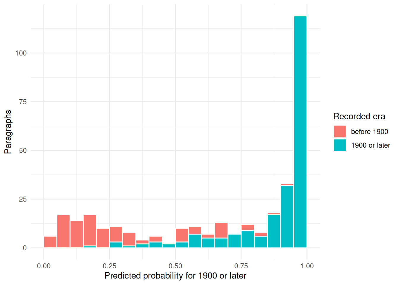
Many scores sit near 0 or 1, and the median is 0.8629 because the later era is the larger class in this test split. Class imbalance matters: the model sees more examples from the larger class, and a naive baseline already gets many rows right by guessing that class.

Choose the cut point

Changing the cut point changes which side absorbs the doubtful cases. This is a decision about how the classifier will be used, not something the fitted model settles alone.

era_thresholds <- tibble(threshold = c(0.40, 0.50, 0.60)) |>
  mutate(
    results = map(threshold, \(cut_point) {
      tfidf_scores |>
        summarise(
          before_1900_sent_late =
            sum(prob_1900_or_later >= cut_point & era == "before 1900"),
          late_sent_before =
            sum(prob_1900_or_later < cut_point & era == "1900 or later"),
          .groups = "drop"
        )
    })
  ) |>
  unnest(results)

knitr::kable(
  era_thresholds,
  col.names = c(
    "Cut point",
    "Earlier paragraphs sent to later label",
    "Later paragraphs sent to earlier label"
  ),
  caption = "Cut-point trade-off for the tf-idf model",
  row.names = FALSE
)

Cut-point trade-off for the tf-idf model

Cut point	Earlier paragraphs sent to later label	Later paragraphs sent to earlier label
0.4	31	7
0.5	28	12
0.6	17	22

At 0.40, seven later-era test paragraphs fall below the cut point. At 0.60, that count rises to 22 while fewer earlier paragraphs move to the later label. A classifier returns a score; a person chooses the cut point that matches the task.

What to remember

• Text classification needs labelled documents and a fixed set of categories.
• The representation step decides which text evidence the model can see.
• A baseline gives the model score a reference point.
• Class imbalance can make easy guesses look better than they are.
• Word-count models ignore order unless order is built into the features.

Sources

• quanteda inaugural corpus documentation
• glmnet package documentation
• textrecipes package documentation