Skip to main content

Using a language model in a reproducible analysis

Treat the model as an instrument: record it, check it against people, and correct for its errors

Learn how to use a local language model to label text inside a research workflow, keep the run reproducible, check it on a random sample reviewed by people, and correct a downstream estimate for the model’s mistakes.

Ruth has the 240 records from the Calder Yard review in lesson 74 and a report to write. A small language model could read every record in an afternoon. Her report does not need the model to be impressive. It needs one number she can defend: what share of the collection is responsive, and how sure she can be.

This page treats the model the way a careful researcher treats any measuring instrument. The instrument is written down before it is used, its readings are saved, a random sample is checked by people, and the final estimate is corrected for the errors that sample reveals. Nothing here is specific to one model. The same steps apply to a hosted model, a local one, or a trained classifier.

Note

The records are the constructed review collection from lesson 74. They are fictional teaching records, and their reference labels were written by the page author when the collection was built. Here those labels play the part of a careful human review.

TipWhat you will learn

This page shows how to:

• decide when a language model is a reasonable instrument for a text task;
• record a model run so another person can repeat it;
• treat saved outputs as the record and reruns as a check;
• compare model labels with a random sample reviewed by people;
• correct an estimate for the model’s errors with that sample; and
• find R tools that support this way of working.

Decide whether a language model is the right instrument

Language models can now annotate, classify, extract, and summarize text well enough to be useful in research. On some annotation tasks they match or beat crowd workers at a small fraction of the cost. Careful replications also find them inconsistent: the same model can do well on one dataset and poorly on the next, and small changes to a prompt’s wording or format can move accuracy by many points.

Three findings shape the advice on this page. First, a model follows a written codebook, with definitions and edge cases, more reliably than a bare category name, and the codebook matters more than clever phrasing. Second, with a few hundred labelled examples for a stable task, a fine-tuned small model often matches or beats prompting a large one, at lower cost and with more stable output. Third, labels are inputs to an analysis rather than findings. Even labels that agree with people most of the time can bias a downstream estimate, because their errors are rarely random.

The earlier lessons still apply. A model does not replace corpus design (lesson 4), a defined unit of analysis, or held-out evaluation (lesson 44). It replaces one coder, and it needs checking like one.

Record the instrument before using it

An instrument record lists everything that decides what the model says. Here that means the model and its exact revision, the prompt, and the decoding settings. The prompt lives in a file, so it has a fingerprint like any other data file. It was written from the review request alone, before the model saw any record, and was not revised after reading the model’s answers.

library(dplyr)
library(ggplot2)
library(jsonlite)
library(purrr)
library(readr)
library(stringr)
library(tibble)
library(tidyr)

source("R/use-nlg.R")
source("R/lesson-figures.R")

hash_lines <- function(path) {
  digest::digest(
    paste(read_lines(path), collapse = "\n"),
    algo = "sha256",
    serialize = FALSE
  )
}

collection_path <- "data/riverton/riverton-review-collection.csv"
prompt_path <- "data/riverton/riverton-llm-review-prompt.json"

records <- read_csv(
  collection_path,
  na = c("", "NA"),
  col_types = cols(
    .default = col_character(),
    reference_responsive = col_logical()
  )
) |>
  select(doc_id, review_request, text, reference_responsive)

prompt <- read_json(prompt_path)
model_record <- nlg_model_manifest() |>
  filter(model_key == "qwen_1_5b_instruct")

cat(prompt$system, "", prompt$user_template, sep = "\n")

You review records for one legal request. Follow the codebook. Reply with one word: yes or no.

Request: {request}

Codebook:
- Answer yes when the record is about hiding safety inspection delays, changing inspection logs, or deleting inspection-related messages for the Calder Yard contract. Vague or indirect wording that asks someone to keep an inspection problem out of a document counts.
- Answer no when the record is about other work, even if it mentions an inspection, a log, or a delay.

Record: {record}

Is this record responsive to the request? Answer yes or no.

Instrument record for the review labels

Instrument	Value
model	Qwen/Qwen2.5-1.5B-Instruct
revision	989aa7980e4cf806f80c7fef2b1adb7bc71aa306
license	Apache-2.0
prompt ID	riverton-review-yes-no-v1
prompt SHA-256	48868d4b581e5a4d0f97eb04278ecdfd0611eafd5f38ec99a5763754417c7366
decoding	greedy: the most likely next token at every step
tokens allowed per answer	3

The model is an open-weight model pinned to one revision, and every runtime file listed in the project’s model manifest is checked against a recorded SHA-256 before it loads. A hosted model can change behind the same name or be retired on the provider’s schedule, so a hosted run needs the dated model version and a saved copy of every answer.

Label every record once and keep the outputs

The builder script data-raw/build-llm-review-labels.R sent this prompt, once per record, to the pinned model and saved every raw answer with the run’s metadata. Rendering this page reads that saved run; it does not relabel the collection. The saved file is the record of what the model said. A rerun later is a check on that record, not a replacement for it.

Before the saved labels are used, the page checks that they still belong to this instrument. If someone edits the prompt, swaps the model, changes the decoding settings, or changes the collection, the check fails and the page stops instead of reporting labels from a different run.

labels_path <- "data/riverton/riverton-llm-review-labels.csv"

cached_labels <- read_csv(
  labels_path,
  na = character(),
  col_types = cols(
    doc_id = col_character(),
    raw_output = col_character(),
    llm_label = col_character(),
    output_tokens = col_integer(),
    ended_by_eos = col_logical()
  )
)

run_record <- read_csv(
  "data/riverton/riverton-llm-review-labels-metadata.csv",
  na = character(),
  col_types = cols(.default = col_character())
)

decoding_settings <- paste(
  "greedy; do_sample = FALSE; num_beams = 1; max_new_tokens = 3;",
  "repetition_penalty = 1"
)

parse_answer <- function(raw_output) {
  first_word <- str_extract(str_to_lower(raw_output), "[a-z]+")
  case_when(
    first_word == "yes" ~ "responsive",
    first_word == "no" ~ "not responsive",
    TRUE ~ "unparsed"
  )
}

cache_checks <- tibble(
  check = c(
    "labels file matches its recorded fingerprint",
    "prompt file and prompt ID match the run",
    "review collection matches the one the run labelled",
    "model ID and revision match the pinned manifest",
    "decoding settings match this page",
    "every saved label matches its raw answer"
  ),
  passed = c(
    hash_lines(labels_path) == run_record$fingerprint,
    hash_lines(prompt_path) == run_record$prompt_sha256 &&
      prompt$prompt_id == run_record$prompt_id,
    hash_lines(collection_path) == run_record$collection_sha256,
    run_record$model_id == model_record$model_id &&
      run_record$revision == model_record$revision,
    run_record$decoding == decoding_settings,
    all(parse_answer(cached_labels$raw_output) == cached_labels$llm_label)
  )
)

The saved run is checked against the instrument record

Check before using the saved labels	Passed
labels file matches its recorded fingerprint	TRUE
prompt file and prompt ID match the run	TRUE
review collection matches the one the run labelled	TRUE
model ID and revision match the pinned manifest	TRUE
decoding settings match this page	TRUE
every saved label matches its raw answer	TRUE

Details recorded by the builder when it labelled the collection

Run detail	Value
created_on	2026-09-25
decoding	greedy; do_sample = FALSE; num_beams = 1; max_new_tokens = 3; repetition_penalty = 1
platform	R version 4.6.1 (2026-06-24 ucrt); Windows 11 x64 (build 26200); Python 3.12.10; torch 2.9.1+cpu; transformers 4.57.6
seconds_per_record	23.16

The model answered yes for 14 records and no for 226. Every answer began with one of the two allowed words. The page decided in advance how to treat any other answer: it counts as not responsive, because the model did not say the record was responsive.

Rerun a few records to test the record

Greedy decoding picks the single most likely token at every step, so the same software on the same machine usually repeats itself. Across machines, library versions, or server batch sizes, small numerical differences can change a choice, and “temperature 0” on a hosted service is not a guarantee. The check below reruns eight records chosen with seed 925, the date the prompt was written, and compares the new answers with the saved ones.

fill_prompt <- function(request, record) {
  prompt$user_template |>
    str_replace(fixed("{request}"), request) |>
    str_replace(fixed("{record}"), record)
}

model <- load_nlg_pipeline("qwen_1_5b_instruct", "text-generation")

ask_model <- function(request, record) {
  chat_prompt <- nlg_chat_prompt(
    model$tokenizer,
    prompt$system,
    fill_prompt(request, record)
  )
  nlg_generate(model, chat_prompt, max_new_tokens = 3L)$text
}

set.seed(925)
rerun <- records |>
  slice_sample(n = 8) |>
  mutate(rerun_output = map2_chr(review_request, text, ask_model)) |>
  left_join(cached_labels |> select(doc_id, raw_output), by = "doc_id") |>
  mutate(identical_answer = rerun_output == raw_output)

Eight saved answers rerun during this render

Record	Text	Saved answer	Answer in this render	Identical
RYD-0106	Use the front tablet for badge photos this week because the kiosk camera flickers. Call me if anything is unclear.	no	no	TRUE
RYD-0167	Chat at noon: The inspector role in the training exercise is assigned to Marcus.	no	no	TRUE
RYD-0026	Forwarding from intake: The Room 104 sink repair note belongs in the maintenance binder.	no	no	TRUE
RYD-0047	Per scheduling: Move the translation cards to the library event folder with the bilingual flyers.	no	no	TRUE
RYD-0179	Reminder: Move the spare chargers beside the loaner laptop case after checking their labels.	no	no	TRUE
RYD-0004	Forwarding from intake: Please refill the badge sleeves before the Tuesday visitor group arrives, then restock the reception tray.	no	no	TRUE
RYD-0076	Please note: Keep the rough yard timeline out of the shared packet today.	no	no	TRUE
RYD-0116	Reminder: Move the donated coats to the storage room this afternoon and keep adult sizes separate.	no	no	TRUE

In this render, 8 of 8 rerun answers match the saved answers exactly. The page does not require all eight to match, because a render on a different computer may differ. It reports what happened, and the estimates below use the saved answers either way.

Check the labels against people on a random sample

A person now reviews a simple random sample of 40 records, drawn so that every record has the same chance of selection. The seed, 2509, was fixed before the first draw, and the sample is drawn once. Random selection is what lets the sample speak for the whole collection; a sample of hand-picked or easy records would not.

sample_size <- 40L

label_levels <- c("not responsive", "responsive")

set.seed(2509)
review_sample <- records |>
  slice_sample(n = sample_size) |>
  left_join(cached_labels |> select(doc_id, llm_label), by = "doc_id") |>
  mutate(
    person_says = factor(
      if_else(reference_responsive, "responsive", "not responsive"),
      levels = label_levels
    ),
    model_says = factor(
      if_else(llm_label == "responsive", "responsive", "not responsive"),
      levels = label_levels
    )
  )

agreement <- review_sample |>
  count(person_says, model_says, name = "records", .drop = FALSE)

Model labels compared with the person’s review on the random sample

Person’s reading	Model says not responsive	Model says responsive
not responsive	33	0
responsive	4	3

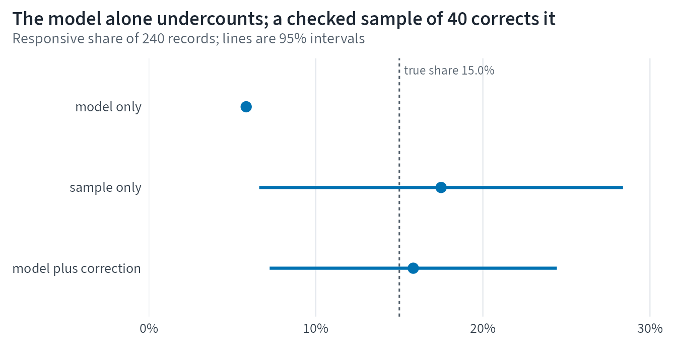
The model and the person agree on 36 of the 40 sampled records. Agreement alone hides which way the errors run. Here every disagreement runs the same way: the model missed 4 responsive records and flagged no record the person called not responsive, so a count of its labels will run low.

Estimate the responsive share without trusting the model blindly

Three estimates of the responsive share are possible:

• Model only: the share of all 240 records the model called responsive. It uses every record but inherits every error the model makes.
• Sample only: the share of the 40 sampled records the person called responsive. It is unbiased but uncertain, because 40 records is a small sample.
• Model plus correction: the model-only share, plus the average difference between the person’s reading and the model’s label on the sample. The sample estimates the model’s average error, and the correction subtracts that estimate.

The third estimate is the difference estimator from survey sampling. In machine learning the same idea is called prediction-powered inference. Over repeated random samples it is unbiased, and its precision depends on how much the difference between the person’s reading and the model’s label varies from record to record. When the model agrees with people on most records, the interval is narrower than the sample alone would give. Each interval below is the estimate plus or minus 1.96 standard errors, with the finite-population correction for sampling 40 of 240 records.

all_records <- nrow(records)

model_flags <- cached_labels |>
  transmute(doc_id, model_flag = as.integer(llm_label == "responsive"))

sample_values <- review_sample |>
  transmute(doc_id, person_flag = as.integer(reference_responsive)) |>
  left_join(model_flags, by = "doc_id") |>
  mutate(difference = person_flag - model_flag)

finite_population_se <- function(values, population_size) {
  sqrt((1 - length(values) / population_size) * var(values) / length(values))
}

model_only <- mean(model_flags$model_flag)
sample_only <- mean(sample_values$person_flag)
corrected <- model_only + mean(sample_values$difference)

estimates <- tibble(
  method = c("model only", "sample only", "model plus correction"),
  estimate = c(model_only, sample_only, corrected),
  standard_error = c(
    0,
    finite_population_se(sample_values$person_flag, all_records),
    finite_population_se(sample_values$difference, all_records)
  )
) |>
  mutate(
    low = pmax(0, estimate - 1.96 * standard_error),
    high = pmin(1, estimate + 1.96 * standard_error)
  )

true_share <- mean(records$reference_responsive)

Three estimates of the responsive share of the collection

Method	Estimated responsive share	95% interval	Uses
model only	5.8%	none: no sampling, but the model’s bias remains	model labels for all 240 records
sample only	17.5%	6.6% to 28.4%	the person’s review of 40 records
model plus correction	15.8%	7.2% to 24.4%	model labels for all 240 records and the review of 40

Because this collection is constructed, the true share is known: 15.0%. A real project would not have this number. It is shown only so the three methods can be judged.

estimate_plot <- estimates |>
  mutate(method = factor(method, levels = rev(estimates$method)))

ggplot(estimate_plot, aes(x = estimate, y = method)) +
  geom_vline(
    xintercept = true_share,
    linetype = "22",
    colour = lesson_colours[["muted"]]
  ) +
  geom_linerange(
    aes(xmin = low, xmax = high),
    linewidth = 1.1,
    colour = lesson_colours[["accent"]]
  ) +
  geom_point(size = 3.2, colour = lesson_colours[["accent"]]) +
  annotate(
    "text",
    x = true_share,
    y = 3.45,
    label = str_c("true share ", scales::percent(true_share, accuracy = 0.1)),
    hjust = -0.05,
    family = lesson_font,
    size = 3.4,
    colour = lesson_colours[["muted"]]
  ) +
  scale_x_continuous(
    labels = scales::label_percent(accuracy = 1),
    limits = c(0, NA),
    expand = expansion(mult = c(0, 0.08))
  ) +
  labs(
    title = estimate_title,
    subtitle = "Responsive share of 240 records; lines are 95% intervals",
    x = NULL,
    y = NULL
  ) +
  theme_lesson(grid = "x")

Figure 1: Three estimates of the responsive share, with 95% intervals, against the true share known only because the collection is constructed.

Repeat the sample to see why the correction works

One sample could be lucky. Drawing the 40-record sample 2,000 more times, with no new model calls, shows how each method behaves in the long run. For each draw, the code repeats the two sample-based estimates and asks whether each interval contains the true share.

set.seed(2510)
repeated <- map(seq_len(2000L), \(draw) {
  sampled <- sample(all_records, sample_size)
  person <- as.integer(records$reference_responsive[sampled])
  difference <- person - model_flags$model_flag[sampled]

  tibble(
    draw = draw,
    method = c("sample only", "model plus correction"),
    estimate = c(mean(person), model_only + mean(difference)),
    standard_error = c(
      finite_population_se(person, all_records),
      finite_population_se(difference, all_records)
    )
  )
}) |>
  list_rbind() |>
  mutate(
    covers_truth = abs(estimate - true_share) <= 1.96 * standard_error
  )

long_run <- repeated |>
  summarise(
    average_estimate = mean(estimate),
    average_interval_width = mean(2 * 1.96 * standard_error),
    coverage = mean(covers_truth),
    .by = method
  )

Two sample-based estimators over 2,000 repeated samples of 40 records

Method	Average estimate	Average interval width	Intervals containing the true share
sample only	15.2%	20.1 points	96.2%
model plus correction	15.2%	16.1 points	92.4%

Both methods average close to the true share. The corrected intervals are narrower, 16.1 percentage points wide on average against 20.1 percentage points for the sample alone, because the model’s labels settle most records and the person only has to measure its misses. They contain the true share in 92.4% of samples, a little short of the nominal 95%, against 96.2% for the sample alone. The shortfall comes from the simple normal-approximation interval, which is rough when the model’s misses are rare in a sample of 40. In 20 of the 2,000 samples none of the misses were drawn, so the corrected interval had no width at all. A larger sample, or an interval built for rare events, would close the gap.

A checklist for model-assisted analysis

• Choose the instrument on purpose. Prefer a rule, a dictionary, or a small trained model when it does the job, and use a language model when the task needs reading that those cannot do.
• Write the codebook and prompt before the first run, store them as a file, and record the file’s fingerprint.
• Pin the model. Record the model name, exact revision or dated version, decoding settings, and software versions. Open weights that you can run yourself make this easier, though they do not remove every source of variation.
• Save every raw output with the ID of the input that produced it.
• Rerun a sample and report how many answers repeat.
• Check the labels against people on a random sample, and report both kinds of error.
• Correct any estimate that uses model labels, with the difference estimator or a related method such as prediction-powered inference or design-based supervised learning.
• Test a model used as a judge the same way before trusting its scores.
• Check structured output for content as well as format. A reply that matches a schema can still hold wrong values.
• Read and rerun code that an assistant wrote, keep a reference calculation for key numbers, and pin the environment.
• Disclose the model’s role using a reporting checklist such as GUIDE-LLM or TRIPOD-LLM.

R tools for this way of working

The packages below were checked on 25 September 2026. Versions change often, so check again before relying on one.

R packages for model-assisted text analysis, checked 25 September 2026

Package	What it does	Runs with local models
ellmer 0.5.0	Chat with model providers, call tools, and extract structured data	Yes, through Ollama
mall 0.2.0	Classify, extract, or score a data frame column row by row	Yes, designed for Ollama
ragnar 0.3.1	Chunk documents, store embeddings, and retrieve passages	Partly; document conversion uses Python
vitals 0.4.0	Evaluate model-based tools, including model-graded scoring	Yes, with any ellmer chat
tidyllm 0.6.0	One tidy interface to several providers	Yes, through Ollama
ipd 0.4.1	Inference on predicted data, including prediction-powered inference	Not needed; it uses saved labels
huggingfaceR 2.1.0	Hugging Face models through Python, used on this site	Yes, fully offline once models are saved

The reference implementation of design-based supervised learning is the dsl package on GitHub, which is not on CRAN.

What to remember

• A language model is an instrument; write down the model, revision, prompt, and settings before using it.
• The saved outputs are the reproducible record; a rerun tests that record.
• A random sample reviewed by people shows how the model errs.
• Correct estimates with that sample; model-only numbers carry the model’s bias.
• The earlier lessons’ rules still apply: provenance, stable IDs, baselines, and held-out evaluation.

Ruth’s report gives the corrected share with its interval, the sample it rests on, and the instrument record, so a reader can check each step.

Sources

• Gilardi, Alizadeh, and Kubli (2023), ChatGPT outperforms crowd workers for text-annotation tasks
• Kristensen-McLachlan et al. (2025), Are chatbots reliable text annotators? Sometimes
• Halterman and Keith, Codebook LLMs: evaluating LLMs as measurement tools for political science concepts
• Törnberg (2024), Best practices for text annotation with large language models
• Edwards and Camacho-Collados (2024), Language models for text classification: is in-context learning enough?
• Sclar et al. (2024), Quantifying language models’ sensitivity to spurious features in prompt design
• Angelopoulos et al. (2023), Prediction-powered inference
• Egami et al. (2023), Using imperfect surrogates for downstream inference
• Salerno et al. (2025), ipd: an R package for conducting inference on predicted data
• Atil et al. (2025), Non-determinism of “deterministic” LLM system settings in hosted environments
• Thinking Machines Lab (2025), Defeating nondeterminism in LLM inference
• Chen, Zaharia, and Zou (2024), How is ChatGPT’s behavior changing over time?
• Palmer, Smith, and Spirling (2024), Using proprietary language models in academic research requires explicit justification
• Bavaresco et al. (2025), LLMs instead of human judges? A large-scale empirical study across 20 NLP evaluation tasks
• Tam et al. (2024), Let me speak freely? A study on the impact of format restrictions on LLM performance
• Bridgeford et al. (2026), Twelve quick tips for AI-assisted coding in science
• Feuerriegel et al. (2026), A reporting checklist for large language models in behavioural science
• Gallifant et al. (2025), The TRIPOD-LLM reporting guideline
• ellmer documentation
• mall documentation
• ragnar documentation
• vitals documentation