Skip to main content

Checking word trends over time

Normalize counts and test the peak

Learn how to track word frequency across speeches while separating durable patterns from one-document spikes.

Nia is preparing a timeline for a classroom wall. She can fit four word paths on the chart, and every path has to be fair to speeches of different lengths.

A raw count would reward long speeches. A rate per thousand alphabetic tokens gives each speech a comparable scale, but a clean-looking line can still be carried by one short document.

TipWhat you will learn

This lesson shows how to:

• count selected words by speech year;
• normalize word counts per thousand alphabetic tokens;
• flag rates from very short speeches;
• recompute each peak after removing its peak speech; and
• compare one trajectory with a permutation null.

Count words by speech

A trend is a pattern over time. Counting alone does not prove one. The first step is still useful: put every speech on the same rate scale so length is not the only driver.

library(dplyr)
library(tidyr)
library(tibble)
library(stringr)
library(tidytext)
library(ggplot2)
library(knitr)

source("R/inaugural-corpus.R")
source("R/permutation-null.R")

paragraphs <- inaugural_paragraphs()

speeches <- paragraphs |>
  summarise(text = paste(paragraph, collapse = "\n"), .by = c(speech_id, year, president, party))

speech_tokens <- speeches |>
  select(speech_id, year, president, text) |>
  unnest_tokens(word, text) |>
  filter(str_detect(word, "^[a-z]+$"))

speech_lengths <- speech_tokens |>
  count(speech_id, year, president, name = "total_alphabetic_tokens")

target_words <- c("america", "freedom", "constitution", "children")
min_tokens_for_rate <- 500L

length_context <- speech_lengths |>
  summarise(
    median_alphabetic_tokens = median(total_alphabetic_tokens),
    minimum_alphabetic_tokens = min(total_alphabetic_tokens)
  )

trend_counts <- speech_tokens |>
  count(speech_id, year, president, word, name = "count") |>
  filter(word %in% target_words) |>
  right_join(
    expand_grid(speech_lengths, word = target_words),
    by = join_by(speech_id, year, president, word)
  ) |>
  mutate(
    count = coalesce(count, 0L),
    per_thousand_alphabetic = count / total_alphabetic_tokens * 1000,
    below_min_tokens = total_alphabetic_tokens < min_tokens_for_rate,
    word = factor(word, levels = target_words)
  ) |>
  arrange(word, year)

trend_summary <- trend_counts |>
  group_by(word) |>
  arrange(desc(per_thousand_alphabetic), year, .by_group = TRUE) |>
  reframe(
    total = sum(count),
    speeches_with_word = sum(count > 0),
    max_rate = round(first(per_thousand_alphabetic), 2),
    max_year = first(year),
    max_count = first(count),
    tokens_at_max = first(total_alphabetic_tokens),
    max_rate_flag = if_else(first(below_min_tokens), "under 500 tokens", "ok"),
    rate_excluding_largest = round(max(per_thousand_alphabetic[-1]), 2),
    year_excluding_largest = year[-1][which.max(per_thousand_alphabetic[-1])],
    guarded_rate_excluding_largest = round(
      max(
        per_thousand_alphabetic[-1][
          total_alphabetic_tokens[-1] >= min_tokens_for_rate
        ]
      ),
      2
    ),
    guarded_year_excluding_largest = year[-1][
      total_alphabetic_tokens[-1] >= min_tokens_for_rate
    ][
      which.max(
        per_thousand_alphabetic[-1][
          total_alphabetic_tokens[-1] >= min_tokens_for_rate
        ]
      )
    ],
    survives_guard = max_rate_flag == "ok" & guarded_rate_excluding_largest >= max_rate * 0.5
  ) |>
  ungroup()

kable(
  trend_summary,
  col.names = c(
    "Word", "Total count", "Speeches with word",
    "Max per 1,000 alphabetic tokens", "Max year",
    "Count in max year", "Alphabetic tokens at max", "Max-rate flag",
    "Rate excluding largest",
    "Year excluding largest", "Guarded rate excluding largest", "Guarded year", "Survives guard"
  ),
  caption = "Summary of four tracked words across 60 speeches",
  row.names = FALSE
)

Summary of four tracked words across 60 speeches

Word	Total count	Speeches with word	Max per 1,000 alphabetic tokens	Max year	Count in max year	Alphabetic tokens at max	Max-rate flag	Rate excluding largest	Year excluding largest	Guarded rate excluding largest	Guarded year	Survives guard
america	166	31	9.62	1993	15	1559	ok	7.41	1793	6.75	1973	TRUE
freedom	175	36	12.35	2005	25	2025	ok	6.84	1957	6.84	1957	TRUE
constitution	207	39	7.41	1793	1	135	under 500 tokens	6.65	1861	6.65	1861	FALSE
children	49	22	3.11	2001	4	1285	ok	2.83	1997	2.83	1997	TRUE

These four words were chosen to illustrate the method. Searching hundreds of words and reporting only the lines that look dramatic would create a multiple-comparisons problem: the search itself would make an unusual-looking line easier to find. A real trend scan must record how many words were tested and adjust its evidence or confirm the result on new documents.

The denominator counts lowercase ASCII alphabetic tokens because the tokenizer filters everything else before measuring speech length. The table says how often each tracked word appears and where it was densest on that stated scale. Rates from speeches under 500 alphabetic tokens are flagged because one occurrence in such a document is at least 2 uses per thousand. The median speech here has about 1,959 alphabetic tokens, so the cutoff catches the smallest denominators without removing most speeches.

Plot the trajectories

A line chart earns its place here because the corpus spans 236 years. Each dot is one speech, and each line connects speeches for one word. Open circles mark rates from speeches under 500 alphabetic tokens.

plot_data <- trend_counts |>
  mutate(word = factor(word, levels = target_words))

ggplot(plot_data, aes(x = year, y = per_thousand_alphabetic, color = word)) +
  geom_line(linewidth = 0.7) +
  geom_point(aes(shape = below_min_tokens), size = 1.6) +
  scale_shape_manual(
    values = c(`FALSE` = 16, `TRUE` = 1),
    labels = c(`FALSE` = "500+ tokens", `TRUE` = "under 500 tokens")
  ) +
  labs(
    x = "Speech year",
    y = "Uses per 1,000 alphabetic tokens",
    color = "Word",
    shape = "Denominator"
  ) +
  theme_minimal()

Figure 1: Uses per thousand alphabetic tokens for four selected words across 60 inaugural addresses.

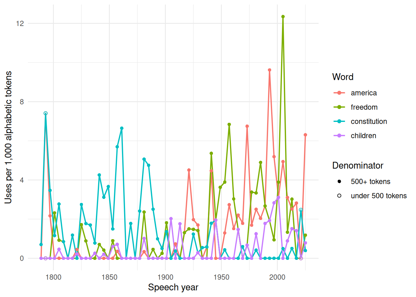
The chart shows word-rate paths, not causes. A rise can reflect changing word choice, changing subject matter, transcription conventions, speech length, or some mix of those. Counts do not split those explanations by themselves.

Test the peak and a null

The largest-contributor check has to use the statistic being reported. Here that statistic is the peak rate, so each word is checked after removing the speech that created its maximum per-thousand value.

A permutation null asks what peak appears after the word occurrences are randomly reassigned. The p-value is the fraction of those shuffled peaks that are at least as high as the observed peak.

constitution_counts <- trend_counts |>
  filter(word == "constitution")

constitution_peak_null <- permutation_null(
  observed = max(constitution_counts$per_thousand_alphabetic),
  replicate_fn = function() {
    assigned_speeches <- sample(
      seq_along(constitution_counts$total_alphabetic_tokens),
      size = sum(constitution_counts$count),
      replace = TRUE,
      prob = constitution_counts$total_alphabetic_tokens
    )
    random_counts <- tabulate(
      assigned_speeches,
      nbins = length(constitution_counts$total_alphabetic_tokens)
    )
    max(random_counts / constitution_counts$total_alphabetic_tokens * 1000)
  },
  replicates = 1000L,
  seed = 5601L,
  alternative = "greater"
)

constitution_peak_null_display <- constitution_peak_null |>
  mutate(across(c(observed, null_mean, null_low, null_high, p_value), \(x) round(x, 3)))

constitution_top_rates <- constitution_counts |>
  arrange(desc(per_thousand_alphabetic), year) |>
  slice_head(n = 5) |>
  transmute(
    speech_id,
    year,
    president,
    count,
    total_alphabetic_tokens,
    per_thousand_alphabetic = round(per_thousand_alphabetic, 2),
    denominator_flag = if_else(below_min_tokens, "under 500 tokens", "ok")
  )

kable(
  constitution_top_rates,
  col.names = c(
    "Speech",
    "Year",
    "President",
    "Count",
    "Alphabetic tokens",
    "Per 1,000 alphabetic tokens",
    "Denominator flag"
  ),
  caption = "The highest constitution rates and their denominators",
  row.names = FALSE
)

The highest constitution rates and their denominators

Speech	Year	President	Count	Alphabetic tokens	Per 1,000 alphabetic tokens	Denominator flag
1793-Washington	1793	George Washington	1	135	7.41	under 500 tokens
1861-Lincoln	1861	Abraham Lincoln	24	3611	6.65	ok
1857-Buchanan	1857	James Buchanan	16	2808	5.70	ok
1881-Garfield	1881	James A. Garfield	15	2963	5.06	ok
1885-Cleveland	1885	Grover Cleveland	8	1684	4.75	ok

kable(
  constitution_peak_null_display,
  col.names = c("Observed", "Null mean", "Null low", "Null high", "p-value", "Replicates", "Alternative"),
  caption = "Permutation null for the constitution peak rate",
  row.names = FALSE
)

Permutation null for the constitution peak rate

Observed	Null mean	Null low	Null high	p-value	Replicates	Alternative
7.407	5.314	3.42	7.426	0.233	1000	greater

The headline problem is visible for constitution. Its maximum rate is 7.41 per thousand alphabetic tokens in 1793, but that speech has only 135 alphabetic tokens. One occurrence creates the peak. After removing that peak speech, the next rate is 6.65 in 1861; with the denominator guard applied, the peak does not survive because the reported maximum came from an under-500-token document. Shuffling the 207 occurrences across fixed speech lengths gives a null mean of 5.31, a 90% interval from 3.42 to 7.43, and p = 0.233. The observed 1793 peak is well within what this shuffle can produce.

Trend methods always draw a line once the analyst picks words and dates. The null asks what peak would appear if the same number of word occurrences landed in speeches according to speech length, with time labels no longer carrying the pattern.

What to remember

• Normalize word counts per thousand alphabetic tokens before comparing speeches.
• Flag rates from very short documents; this lesson uses a 500-token cutoff.
• The four tracked words have different coverage across the 60 speeches.
• constitution peaks in 1793 only because 1 occurrence sits in a 135-word speech.
• Word-rate change can mix word choice, subject matter, transcription, and length.

Use trend charts to ask better reading questions, then test whether the pattern survives the obvious stress check.

Sources

• tidytext reference for tokenizing text
• Pechenick, Danforth, and Dodds on limits of word-frequency inference
• ggplot2 documentation
• quanteda inaugural address corpus documentation