library(dplyr)
library(tibble)
library(stringr)
library(readr)
library(quanteda)
library(word2vec)
library(ggplot2)

source("R/inaugural-corpus.R")

within_tolerance <- function(observed, expected, tolerance = 1e-4) {
  abs(observed - expected) < tolerance
}

metadata <- read_csv(
  "data/word2vec/word2vec-metadata.csv",
  na = character(),
  col_types = cols(
    field = col_character(),
    value = col_character()
  )
)
metadata_values <- setNames(metadata$value, metadata$field)

paragraphs <- inaugural_paragraphs()
training_tokens <- tokens(
  paragraphs$paragraph,
  remove_punct = TRUE,
  remove_numbers = TRUE
) |>
  tokens_tolower()

model <- word2vec::read.word2vec("data/word2vec/inaugural-word2vec.bin")
embedding_matrix <- as.matrix(model)
punctuation_rows <- rownames(embedding_matrix)[grepl("[[:punct:]]", rownames(embedding_matrix))]

training_summary <- tibble(
  item = c(
    "training documents",
    "tokens after cleanup",
    "vocabulary rows",
    "dimensions",
    "punctuation rows",
    "unique word pairs"
  ),
  value = c(
    metadata_values[["training_documents"]],
    metadata_values[["training_tokens"]],
    metadata_values[["vocabulary_rows"]],
    metadata_values[["dimensions"]],
    metadata_values[["punctuation_rows"]],
    metadata_values[["unique_pairs"]]
  )
)

hyperparameter_table <- tibble(
  setting = c("algorithm", "dimensions", "window", "iterations", "minimum count", "threads"),
  value = metadata_values[c("algorithm", "dimensions", "window", "iterations", "minimum_count", "threads")]
)

model_fingerprint <- tibble(
  field = c("generator", "model SHA-256", "reproducibility note"),
  value = metadata_values[c("generator", "sha256_model", "reproducibility")]
)
Training word vectors
Check whether neighbours carry information
similarity
word embeddings
inaugural addresses
Learn how distributed word representations are trained from local context and why a small corpus can make neighbour lists look better than they are.
A curator wants to tag a speech archive without reading every paragraph. She asks which words sit near freedom, union, and peace in the language of the collection.
A table of neighbours appears quickly. It looks meaningful, but every word-vector model can return a nearest neighbour for any word it kept.
A distributed word representation is one numeric vector per word, learned from the words that appear near it. This lesson loads one saved local model, then checks whether an easy related pair separates from arbitrary pairs.
TipWhat you will learn
This lesson shows how to:
- read a pinned word2vec skip-gram model;
- inspect the preprocessing and training settings stored with it;
- explain why the fitted model is saved rather than trained during render;
- compare an expected related pair with random pairs; and
- summarize the full distribution of cosine similarities.
Load one saved word2vec model
Word2vec comes from work by Mikolov and colleagues on learning word vectors from nearby words. The skip-gram version uses the current word to predict words in its window. The R package splits input on whitespace, so the training strings should already be lowercased with punctuation and numbers removed.
| Item | Value |
|---|---|
| training documents | 1377 |
| tokens after cleanup | 134419 |
| vocabulary rows | 2709 |
| dimensions | 50 |
| punctuation rows | 1 |
| unique word pairs | 3667986 |
| Setting | Value |
|---|---|
| algorithm | skip-gram |
| dimensions | 50 |
| window | 5 |
| iterations | 5 |
| minimum count | 5 |
| threads | 1 |
| Field | Value |
|---|---|
| generator | data-raw/build-word2vec-model.R |
| model SHA-256 | b182100ecb33cb339f16fdf5df5cea783dd113843a3a89e7e65393b921e448dd |
| reproducibility note | word2vec is not bitwise reproducible on this package version. Across five fits with the same seed the neighbour order changed every time, so this model is trained once here and committed. |
The metadata records 1,377 training documents, 134,419 cleaned tokens, 2,709 vocabulary rows, and 3,667,986 unique word pairs. It also records one punctuation row, the trainer’s </s> marker. Punctuation was removed before training, so forms such as peace. and peace, do not compete with peace.
The same training code with the same seed and threads = 1L produced neighbour lists in a different order on each fit. The similarity values moved only slightly, about 0.03 here, but the ranking changed. This page loads one saved fit, and the metadata records its SHA-256 fingerprint. A result you cannot reproduce is a result you cannot check; pinning the artefact is the normal fix when exact words will be printed.
Print neighbours, then distrust the glow
A nearest-neighbour list returns the words with highest cosine similarity to a query word. Cosine similarity compares vector direction; larger values mean closer under the trained representation.
nearest_words <- function(word, n = 6L) {
  predict(model, newdata = word, type = "nearest", top_n = n)[[1]] |>
    as_tibble() |>
    mutate(
      similarity_band = case_when(
        similarity >= 0.8 ~ "0.80 or higher",
        similarity >= 0.7 ~ "0.70 to 0.79",
        TRUE ~ "below 0.70"
      )
    )
}

neighbour_table <- bind_rows(
  nearest_words("union") |>
    mutate(query = "union"),
  nearest_words("freedom") |>
    mutate(query = "freedom"),
  nearest_words("peace") |>
    mutate(query = "peace")
) |>
  select(query, neighbour = term2, similarity, similarity_band, rank)

expected_neighbours <- c(
  "texas", "attachment", "system", "jurisdiction", "confederation", "communities",
  "human", "evil", "mankind", "dignity", "civilization", "ancient",
  "friendship", "lasting", "world", "cultivate", "amity", "prosperity"
)| Query | Nearest word | Cosine similarity | Cosine similarity band | Rank |
|---|---|---|---|---|
| union | texas | 0.921 | 0.80 or higher | 1 |
| union | attachment | 0.919 | 0.80 or higher | 2 |
| union | system | 0.919 | 0.80 or higher | 3 |
| union | jurisdiction | 0.918 | 0.80 or higher | 4 |
| union | confederation | 0.914 | 0.80 or higher | 5 |
| union | communities | 0.914 | 0.80 or higher | 6 |
| freedom | human | 0.918 | 0.80 or higher | 1 |
| freedom | evil | 0.914 | 0.80 or higher | 2 |
| freedom | mankind | 0.908 | 0.80 or higher | 3 |
| freedom | dignity | 0.895 | 0.80 or higher | 4 |
| freedom | civilization | 0.894 | 0.80 or higher | 5 |
| freedom | ancient | 0.893 | 0.80 or higher | 6 |
| peace | friendship | 0.896 | 0.80 or higher | 1 |
| peace | lasting | 0.886 | 0.80 or higher | 2 |
| peace | world | 0.883 | 0.80 or higher | 3 |
| peace | cultivate | 0.881 | 0.80 or higher | 4 |
| peace | amity | 0.865 | 0.80 or higher | 5 |
| peace | prosperity | 0.863 | 0.80 or higher | 6 |
Some neighbours look plausible. That is not enough. A neighbour list always returns something, and a fluent label can make a weak signal feel stronger than it is. Pinning the file makes the printed words checkable; it does not make the small model trustworthy by itself.
Show the similarity distribution
The distribution below uses every unique word pair in the cleaned vocabulary. It also marks the freedom / liberty pair with a vertical line.
normalized_embeddings <- embedding_matrix / sqrt(rowSums(embedding_matrix^2))
word_similarity_matrix <- tcrossprod(normalized_embeddings)
diag(word_similarity_matrix) <- NA_real_
word_similarities <- word_similarity_matrix[upper.tri(word_similarity_matrix)]
freedom_liberty_percentile <- mean(word_similarities <= freedom_liberty_cosine)

similarity_summary <- tibble(
  statistic = c("word pairs", "median", "95th percentile", "freedom / liberty percentile"),
  value = c(
    length(word_similarities),
    median(word_similarities),
    as.numeric(quantile(word_similarities, 0.95)),
    freedom_liberty_percentile
  )
)| Statistic | Value |
|---|---|
| word pairs | 3667986 |
| median | 0.794 |
| 95th percentile | 0.935 |
| freedom / liberty percentile | 0.444 |
freedom / liberty sits at the 44th percentile of the full pairwise distribution in this saved model. The pair was chosen to be easy, yet it lands below the median pair.
Show the plotting code
source("R/lesson-figures.R")

plot_similarities <- tibble(cosine_similarity = word_similarities)

ggplot(plot_similarities, aes(x = cosine_similarity)) +
  geom_histogram(
    bins = 40,
    boundary = 0,
    fill = lesson_colours[["context"]],
    colour = lesson_colours[["paper"]]
  ) +
  geom_vline(
    xintercept = freedom_liberty_cosine,
    linewidth = 0.9,
    linetype = "22",
    colour = lesson_colours[["contrast"]]
  ) +
  annotate(
    "text",
    x = freedom_liberty_cosine,
    y = Inf,
    label = sprintf("freedom / liberty\n%.2f", freedom_liberty_cosine),
    hjust = 1.08,
    vjust = 1.4,
    lineheight = 0.95,
    family = lesson_font,
    size = 3.6,
    colour = lesson_text_colours[["contrast"]]
  ) +
  scale_y_continuous(labels = scales::label_comma()) +
  labs(
    title = "Many arbitrary word pairs sit above an easy related pair",
    subtitle = "Cosine similarity for every pair of words kept by the pinned word2vec model",
    x = "Cosine similarity",
    y = "Word pairs"
  ) +
  theme_lesson(grid = "y")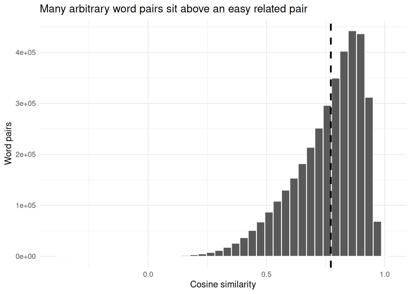
Published embeddings are trained on billions of tokens. Large training text gives the model many more contexts for separating near neighbours from accidental neighbours.
What to remember
- A word2vec model gives one vector to each kept word.
- The pinned model used skip-gram, 50 dimensions, window 5, 5 iterations, minimum count 5, and one thread.
- The word2vec package expects text that is already cleaned before whitespace splitting.
- Neighbour lists need a pinned artefact when exact words are printed.
- In this saved fit, even
freedom / libertylands below the median of all pairwise similarities.
The curator keeps the neighbour table as a prompt for reading, not as evidence that the archive has revealed its themes.