Skip to main content

Counting nearby words with n-grams

See why phrase counts get sparse fast

Learn how bigrams and trigrams count adjacent tokens in the Riverton sentences and why most of them appear only once.

Repeated words such as training stand out in the Riverton Workforce Lab’s short job-board lines and flyer headings. The harder question is whether neighbouring word pairs tell a clearer story.

The coordinator tries a simple phrase count before trusting it. If most phrases appear once, the list may describe these 28 sentences closely while helping less with new documents.

Note

The Riverton Workforce Lab, its job board, and its training flyer are fictional and were created for teaching.

TipWhat you will learn

This lesson shows how to:

• define an n-gram as a run of adjacent tokens;
• build bigrams and trigrams with tidytext;
• count repeated n-grams in the Riverton sentences;
• measure how many n-grams appear once; and
• explain why phrase vocabularies can generalise badly from small data.

Load the sentences

This setup chunk reads the sentence file, prepares small tables, builds n-grams with tidytext, and draws one summary chart. A tibble is a table that prints its size and column types.

library(readr)
library(dplyr)
library(tibble)
library(tidyr)
library(stringr)
library(tidytext)
library(ggplot2)

sentences <- read_csv(
  "data/workforce/workforce_sentences.csv",
  na = character(),
  col_types = cols(
    sentence_id = col_character(),
    document_id = col_character(),
    source_line = col_character(),
    text = col_character(),
    reference_label = col_character(),
    uncertainty = col_character(),
    annotator_id = col_character(),
    rationale = col_character(),
    codebook_version = col_character(),
    codebook_hash = col_character(),
    derived = col_character(),
    transformation = col_character()
  )
)

source_counts <- sentences |>
  mutate(source = if_else(document_id == "F001", "training flyer", "job details")) |>
  count(source, name = "rows")

knitr::kable(
  source_counts,
  col.names = c("Source", "Rows"),
  caption = "The 28 Riverton sentences by source",
  row.names = FALSE
)

The 28 Riverton sentences by source

Source	Rows
job details	22
training flyer	6

The file is small enough to inspect by eye. That convenience is also the reason its phrase counts should be treated as local examples.

Build adjacent-word phrases

An n-gram is a run of n adjacent tokens. A unigram has one token, a bigram has two, and a trigram has three. These counts use the same token rule as Lesson 15: lowercase the text and drop punctuation. Because each row here is one sentence, no n-gram spans two sentences; a file with whole documents in rows would need a different check.

make_ngrams <- function(n) {
  if (identical(n, 1L)) {
    sentences |>
      select(sentence_id, text) |>
      unnest_tokens(output = ngram, input = text, token = "words") |>
      filter(!is.na(ngram))
  } else {
    sentences |>
      select(sentence_id, text) |>
      unnest_tokens(output = ngram, input = text, token = "ngrams", n = n) |>
      filter(!is.na(ngram))
  }
}

short_for_trigrams <- make_ngrams(1L) |>
  count(sentence_id, name = "tokens") |>
  filter(tokens < 3L)

bigrams <- make_ngrams(2L) |>
  count(ngram, name = "frequency", sort = TRUE)
trigrams <- make_ngrams(3L) |>
  count(ngram, name = "frequency", sort = TRUE)

top_phrases <- bind_rows(
  bigrams |>
    slice_head(n = 8) |>
    mutate(kind = "bigram"),
  trigrams |>
    slice_head(n = 8) |>
    mutate(kind = "trigram")
) |>
  select(kind, ngram, frequency)

knitr::kable(
  top_phrases,
  col.names = c("N-gram type", "N-gram", "Frequency"),
  caption = "The most frequent bigrams and trigrams in the 28 sentences",
  row.names = FALSE
)

The most frequent bigrams and trigrams in the 28 sentences

N-gram type	N-gram	Frequency
bigram	is required	4
bigram	training is	3
bigram	are required	2
bigram	experience is	2
bigram	is preferred	2
bigram	is provided	2
bigram	no prior	2
bigram	shifts are	2
trigram	training is provided	2
trigram	12 week training	1
trigram	a daytime schedule	1
trigram	a high school	1
trigram	a medical records	1
trigram	a paid apprenticeship	1
trigram	a portfolio is	1
trigram	a valid driver’s	1

The sentence Evening classes has only two tokens, so it has no trigram. The code drops that empty result before counting. The most frequent bigram is is required, with 4 appearances, and the most frequent trigram is training is provided, with 2.

Measure the sparsity

Sparsity means that many possible items have no examples or only one example. The general reason is arithmetic, not this particular table. Each new word adds at most one new word type, but it can also add a new pair and a new triple; the set of pairs a vocabulary could form grows faster than the vocabulary itself. The Riverton counts below illustrate that argument rather than prove it.

unigrams <- make_ngrams(1L) |>
  count(ngram, name = "frequency", sort = TRUE)

ngram_counts <- list(unigrams, bigrams, trigrams)

ngram_summary <- tibble(
  n = 1:3,
  name = c("unigrams", "bigrams", "trigrams"),
  distinct_items = vapply(ngram_counts, nrow, integer(1)),
  seen_once = vapply(
    ngram_counts,
    \(counts) sum(counts$frequency == 1L),
    integer(1)
  ),
  seen_once_label = str_c(seen_once, "/", distinct_items)
)

knitr::kable(
  ngram_summary,
  col.names = c("n", "Unit", "Distinct units", "Seen once", "Seen-once fraction"),
  caption = "Distinct n-grams and one-time n-grams in the Riverton sentences",
  row.names = FALSE
)

Distinct n-grams and one-time n-grams in the Riverton sentences

n	Unit	Distinct units	Seen once	Seen-once fraction
1	unigrams	96	72	72/96
2	bigrams	112	102	102/112
3	trigrams	96	95	95/96

The 28 sentences contain 96 distinct unigrams, 112 distinct bigrams, and 96 distinct trigrams. The seen-once fractions are 72/96 for unigrams, 102/112 for bigrams, and 95/96 for trigrams. These numbers describe only this teaching corpus.

plot_data <- ngram_summary |>
  transmute(
    name,
    seen_once_share = seen_once / distinct_items,
    seen_once_label
  )

ggplot(plot_data, aes(x = name, y = seen_once_share)) +
  geom_col(fill = "#4C78A8") +
  geom_text(aes(label = seen_once_label), vjust = -0.4) +
  labs(
    x = NULL,
    y = "Share seen once"
  ) +
  scale_y_continuous(labels = \(value) str_c(round(value * 100), "%"), limits = c(0, 1)) +
  theme_minimal()

Figure 1: Share of distinct n-grams seen once in the 28 Riverton sentences.

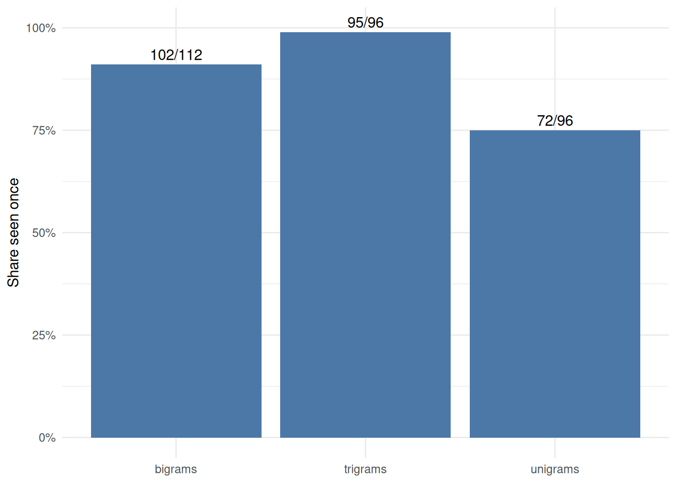
The chart focuses on the quantity the table asks the reader to compare: how much of each list appears only once.

What to remember

• An n-gram counts adjacent tokens after a chosen token rule.
• The Riverton rows contain 112 distinct bigrams and 96 distinct trigrams.
• A two-token sentence contributes no trigram.
• Counts from 28 sentences illustrate sparsity; they do not estimate phrase use in workforce writing.

Report the repeated phrases as local clues, then stop. The useful result here is a small list of repeats paired with a warning about sparse phrase counts.

Sources

• tidytext documentation for unnest_tokens()
• tokenizers documentation for n-gram tokenizers
• ggplot2 documentation