Skip to main content

Measuring distance between texts

Compare string distance with vector distance

Learn how string and vector distances answer different similarity questions, and why raw-count Euclidean distance tracks document length.

A library volunteer receives two boxes of index cards. One box has typed names with small spelling errors, and the other has paragraphs from speeches.

The word “similar” is doing two jobs. Matching a mistyped name is not the same task as comparing the vocabulary of two paragraphs.

A distance measure turns a comparison into a number. Small distance means close. The hard part is choosing a distance that matches the question.

TipWhat you will learn

This lesson shows how to:

• compare edit distance and Jaro-Winkler distance for names;
• build paragraph vectors from word counts;
• compare cosine, Euclidean, and Jaccard distance;
• test whether a distance mostly tracks text length; and
• explain why the same data can give different rankings.

Compare strings directly

String distance compares characters. Levenshtein distance counts edits: insertions, deletions, and substitutions. Jaro-Winkler distance gives extra credit to strings that share an early prefix, which often helps with names.

library(dplyr)
library(tibble)
library(stringr)
library(stringdist)
library(quanteda)
library(Matrix)
library(ggplot2)
library(knitr)

source("R/permutation-null.R")

within_tolerance <- function(observed, expected, tolerance = 1e-3) {
  abs(observed - expected) < tolerance
}

name_matches <- tibble(
  recorded = c("Jonson", "Jonson", "Martha", "Martha", "Stevenson", "Stevenson"),
  candidate = c("Johnson", "Jansen", "Marta", "Marsha", "Stephenson", "Steven")
) |>
  mutate(
    levenshtein = stringdist(recorded, candidate, method = "lv"),
    jaro_winkler = stringdist(recorded, candidate, method = "jw", p = 0.1),
    levenshtein_rank = rank(levenshtein, ties.method = "first"),
    jaro_winkler_rank = rank(jaro_winkler, ties.method = "first")
  )

stevenson_rows <- name_matches |>
  filter(recorded == "Stevenson")

kable(
  name_matches |>
    mutate(jaro_winkler = round(jaro_winkler, 4)),
  col.names = c("Recorded", "Candidate", "Levenshtein", "Jaro-Winkler", "Levenshtein rank", "Jaro-Winkler rank"),
  caption = "Two string distances rank the same candidate names differently",
  row.names = FALSE
)

Two string distances rank the same candidate names differently

Recorded	Candidate	Levenshtein	Jaro-Winkler	Levenshtein rank	Jaro-Winkler rank
Jonson	Johnson	1	0.0381	1	2
Jonson	Jansen	2	0.2000	4	6
Martha	Marta	1	0.0333	2	1
Martha	Marsha	1	0.0778	3	5
Stevenson	Stephenson	2	0.0726	5	4
Stevenson	Steven	3	0.0667	6	3

For Stevenson, Levenshtein picks Stephenson because it needs fewer edits. Jaro-Winkler picks Steven because the shared opening is strong. A name-matching project has to choose the error pattern it cares about.

Build paragraph vectors

A vector is a row of numbers. In a document-feature matrix, each row is a paragraph and each column is a word feature. The entry says how many times that word appears in that paragraph.

source("R/inaugural-corpus.R")

paragraphs <- inaugural_paragraphs()

paragraph_tokens <- tokens(
  paragraphs$paragraph,
  remove_punct = TRUE,
  remove_numbers = TRUE
) |>
  tokens_tolower()

paragraph_dfm <- dfm(paragraph_tokens)
docnames(paragraph_dfm) <- paragraphs$paragraph_id

count_matrix <- as(paragraph_dfm, "dgCMatrix")
token_lengths <- Matrix::rowSums(count_matrix)
squared_lengths <- Matrix::rowSums(count_matrix^2)
dot_products <- as.matrix(Matrix::tcrossprod(count_matrix))

euclidean_squared <- outer(squared_lengths, squared_lengths, "+") - 2 * dot_products
euclidean_squared[euclidean_squared < 0 & euclidean_squared > -1e-8] <- 0
euclidean_distance <- sqrt(euclidean_squared)

vector_norms <- sqrt(squared_lengths)
cosine_similarity <- dot_products / outer(vector_norms, vector_norms)
cosine_distance <- 1 - cosine_similarity

binary_matrix <- Matrix::drop0(count_matrix)
binary_matrix@x <- rep(1, length(binary_matrix@x))
feature_counts <- Matrix::rowSums(binary_matrix)
intersections <- as.matrix(Matrix::tcrossprod(binary_matrix))
unions <- outer(feature_counts, feature_counts, "+") - intersections
jaccard_distance <- 1 - intersections / unions

pair_index <- which(upper.tri(euclidean_distance), arr.ind = TRUE)
pair_distances <- tibble(
  first = pair_index[, 1],
  second = pair_index[, 2],
  length_difference = abs(token_lengths[first] - token_lengths[second]),
  euclidean = euclidean_distance[pair_index],
  cosine = cosine_distance[pair_index],
  jaccard = jaccard_distance[pair_index],
  first_speech = paragraphs$speech_id[first],
  second_speech = paragraphs$speech_id[second]
)

kable(
  tibble(
    item = c("Paragraphs", "Speeches", "People", "Features", "Paragraph pairs"),
    value = c(nrow(paragraphs), n_distinct(paragraphs$speech_id), n_distinct(paragraphs$president), nfeat(paragraph_dfm), nrow(pair_distances))
  ),
  col.names = c("Item", "Value"),
  caption = "Paragraph vectors built from the inaugural-address corpus",
  row.names = FALSE
)

Paragraph vectors built from the inaugural-address corpus

Item	Value
Paragraphs	1377
Speeches	60
People	40
Features	9327
Paragraph pairs	947376

The matrix has 1,377 paragraph rows and 9,327 word columns. Each paragraph becomes a point in a high-dimensional space.

Compare three vector distances

Euclidean distance measures straight-line distance between count vectors. Cosine distance compares direction, so multiplying a paragraph vector by the same constant leaves its cosine direction unchanged. Jaccard distance uses word presence and ignores repeated counts.

length_correlations <- pair_distances |>
  summarise(
    `Euclidean distance` = cor(euclidean, length_difference),
    `Cosine distance` = cor(cosine, length_difference),
    `Jaccard distance` = cor(jaccard, length_difference)
  ) |>
  tidyr::pivot_longer(
    everything(),
    names_to = "distance",
    values_to = "correlation_with_length_difference"
  )

same_speech_examples <- pair_distances |>
  mutate(
    first_paragraph = paragraphs$paragraph_id[first],
    second_paragraph = paragraphs$paragraph_id[second],
    first_length = as.integer(token_lengths[first]),
    second_length = as.integer(token_lengths[second])
  ) |>
  filter(first_speech == second_speech) |>
  arrange(desc(length_difference), euclidean) |>
  slice_head(n = 3) |>
  transmute(
    first_paragraph,
    second_paragraph,
    speech = first_speech,
    first_length,
    second_length,
    length_difference = as.integer(length_difference),
    euclidean = round(euclidean, 2),
    cosine = round(cosine, 3),
    jaccard = round(jaccard, 3)
  )

kable(
  length_correlations |>
    mutate(correlation_with_length_difference = round(correlation_with_length_difference, 3)),
  col.names = c("Distance", "Correlation with length difference"),
  caption = "Raw-count distance compared with paragraph length difference",
  row.names = FALSE
)

Raw-count distance compared with paragraph length difference

Distance	Correlation with length difference
Euclidean distance	0.951
Cosine distance	-0.268
Jaccard distance	0.275

kable(
  same_speech_examples,
  col.names = c("First paragraph", "Second paragraph", "Speech", "First length", "Second length", "Length difference", "Euclidean", "Cosine", "Jaccard"),
  caption = "Long and short paragraphs from the same speech can be far apart under Euclidean distance",
  row.names = FALSE
)

Long and short paragraphs from the same speech can be far apart under Euclidean distance

First paragraph	Second paragraph	Speech	First length	Second length	Length difference	Euclidean	Cosine	Jaccard
1841-Harrison-p10	1841-Harrison-p22	1841-Harrison	984	69	915	147.46	0.330	0.936
1841-Harrison-p10	1841-Harrison-p25	1841-Harrison	984	80	904	145.87	0.304	0.942
1841-Harrison-p10	1841-Harrison-p11	1841-Harrison	984	94	890	142.01	0.229	0.924

The Euclidean correlation with length difference is 0.951, a strong warning that raw-count distance is mostly measuring paragraph size. The cosine correlation is negative, -0.268, because longer paragraphs share many ordinary words with other long paragraphs. That matters for this corpus: nineteenth-century paragraphs are longer than later paragraphs, so a length-shaped method can echo the era pattern seen in the corpus lessons.

same_speech_observed <- pair_distances |>
  filter(first_speech == second_speech) |>
  summarise(mean_cosine_distance = mean(cosine)) |>
  pull(mean_cosine_distance)

speech_labels <- paragraphs$speech_id
same_speech_null <- permutation_null(
  observed = same_speech_observed,
  replicate_fn = function() {
    shuffled_labels <- sample(speech_labels)
    pair_distances |>
      filter(shuffled_labels[first] == shuffled_labels[second]) |>
      summarise(mean_cosine_distance = mean(cosine)) |>
      pull(mean_cosine_distance)
  },
  replicates = 1000L,
  seed = 5902L,
  alternative = "less"
)

kable(
  same_speech_null |>
    mutate(across(where(is.numeric), ~ round(.x, 3))),
  col.names = c("Observed", "Null mean", "Null 5th pct", "Null 95th pct", "p-value", "Replicates", "Alternative"),
  caption = "Same-speech paragraph cosine distance compared with shuffled speech labels",
  row.names = FALSE
)

Same-speech paragraph cosine distance compared with shuffled speech labels

Observed	Null mean	Null 5th pct	Null 95th pct	p-value	Replicates	Alternative
0.569	0.577	0.573	0.581	0.003	1000	less

A distance formula will fill a matrix for any paragraphs it receives. The permutation check asks whether paragraphs from the same speech are closer than a label shuffle would produce. Here they are, but the raw-count Euclidean result is still dominated by length.

set.seed(5901)
plot_pairs <- pair_distances |>
  slice_sample(n = 3000) |>
  tidyr::pivot_longer(
    c(euclidean, cosine, jaccard),
    names_to = "distance",
    values_to = "value"
  )

ggplot(plot_pairs, aes(x = length_difference, y = value)) +
  geom_point(alpha = 0.18, size = 0.7) +
  facet_wrap(~distance, scales = "free_y") +
  labs(
    x = "Difference in paragraph length, in tokens",
    y = "Distance",
    title = "Raw Euclidean distance mostly follows length"
  ) +
  theme_minimal()

Figure 1: Length difference and distance for a deterministic sample of paragraph pairs.

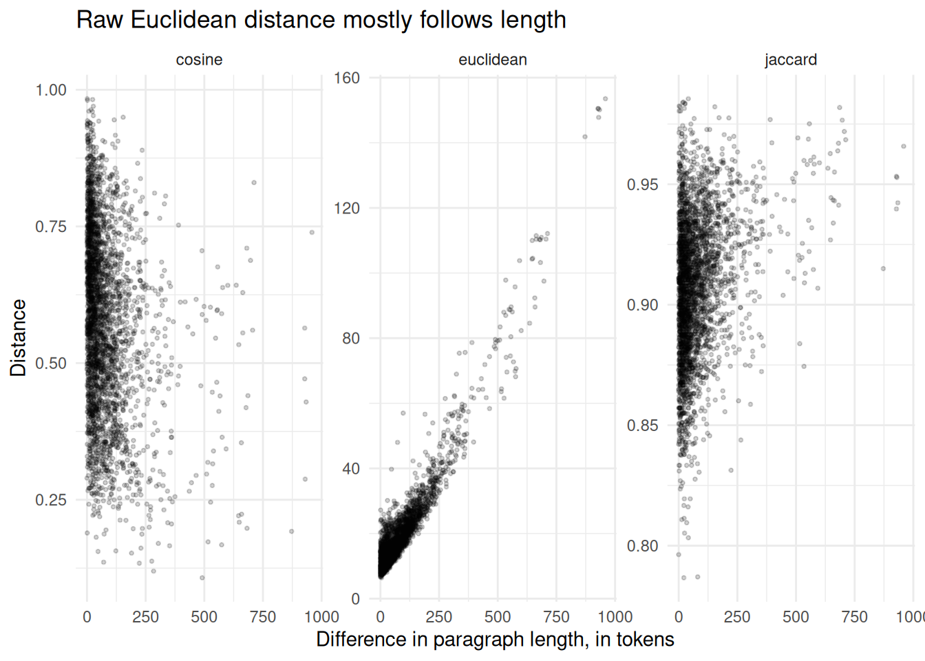
The plot turns the correlation into a visible warning. A long paragraph and a short paragraph can look far apart under raw-count Euclidean distance even when they come from the same speech.

What to remember

• String distance compares character sequences.
• Vector distance compares numeric representations of text.
• Levenshtein and Jaro-Winkler can rank the same name candidates differently.
• On these paragraph counts, Euclidean distance correlates 0.951 with length difference.
• Cosine distance compares direction, which reduces the length problem for raw counts.

The volunteer keeps two labels on the boxes: spelling repair for names, representation choice for paragraphs.

Sources

• stringdist package reference
• quanteda tokens documentation
• United States copyright guidance for government works