suppressPackageStartupMessages({
  library(dplyr)
  library(tibble)
  library(stringr)
  library(tidyr)
  library(stopwords)
  library(ggplot2)
  library(rsample)
  library(recipes)
  library(textrecipes)
  library(parsnip)
  library(workflows)
  library(yardstick)
  library(broom)
  library(glmnet)
})

source("R/inaugural-corpus.R")
paragraphs <- inaugural_paragraphs()

set.seed(4301)
era_split <- group_initial_split(paragraphs, group = speech_id, prop = 0.75)
era_training <- training(era_split)
era_testing <- testing(era_split)

era_recipe <- recipe(era ~ paragraph, data = era_training) |>
  step_tokenize(paragraph) |>
  step_stopwords(paragraph) |>
  step_tokenfilter(paragraph, max_tokens = 500) |>
  step_tfidf(paragraph)

era_model <- logistic_reg(penalty = 0.01, mixture = 0) |>
  set_engine("glmnet")

era_workflow <- workflow() |>
  add_recipe(era_recipe) |>
  add_model(era_model)

set.seed(4302)
era_fitted <- fit(era_workflow, data = era_training)

held_out_predictions <- predict(era_fitted, era_testing) |>
  bind_cols(era_testing |> select(era))

held_out_accuracy <- accuracy(
  held_out_predictions,
  truth = era,
  estimate = .pred_class
) |>
  pull(.estimate)

era_length_summary <- paragraphs |>
  group_by(era) |>
  summarise(
    paragraphs = n(),
    median_words = median(paragraph_words),
    .groups = "drop"
)Monitoring models
Watch a deployed text model after the first score
model development
monitoring
model drift
Learn how to check model performance across time slices and why changing labels can make an old score misleading.
A dashboard turns green on launch day. The model passed its test, the API is ready, and a queue of paragraphs can finally be scored.
Three months later, the queue is different. The words are familiar, the file format still works, and the old test score is still printed in the deployment record. None of that proves the model is doing the same job.
Monitoring asks what changed after deployment. It can watch the text arriving, and when checked labels arrive, it can watch the score.
TipWhat you will learn
This lesson shows how to:
- score a fitted text model across time slices;
- read held-out slice scores without treating them as a new train/test study;
- check input drift when labels are late or missing;
- define concept drift in plain language;
- explain why a fixed party text model needs fresh evidence; and
- name what monitoring can and cannot see.
Refit the era model
For a monitoring lesson, we replay the corpus as if labeled paragraphs arrived from different periods. The model is the same penalized logistic regression with tf-idf features. The split seed is 4301, and the fit seed is 4302.
| Item | Value |
|---|---|
| paragraphs | 1377.0000 |
| held-out paragraphs | 335.0000 |
| held-out accuracy | 0.8209 |
The held-out score is still the evaluation score. Any slice score below uses only those 335 held-out paragraphs, never rows from the training side.
Score held-out time slices
A monitoring slice is a subset watched on its own, such as a month, region, source, or time period. Here the slices are half-centuries. This is already a trap, because the label era is derived from the year. A time slice contains almost only one label, so its score is one-class recall rather than overall performance.
period_breaks <- c(1780, 1849, 1899, 1949, 1999, 2030)
period_levels <- c(
  "1789-1849",
  "1850-1899",
  "1900-1949",
  "1950-1999",
  "2000-2025"
)

held_out_by_period <- held_out_predictions |>
  bind_cols(era_testing |> select(paragraph_id, year, paragraph)) |>
  mutate(
    period = cut(
      year,
      breaks = period_breaks,
      labels = period_levels,
      right = TRUE
    )
  )

label_counts <- held_out_by_period |>
  count(period, era, name = "labels") |>
  complete(
    period = factor(period_levels, levels = period_levels),
    era = levels(paragraphs$era),
    fill = list(labels = 0L)
  )

period_accuracy <- label_counts |>
  group_by(period) |>
  summarise(
    held_out_paragraphs = sum(labels),
    before_1900 = sum(labels[era == "before 1900"]),
    later_1900 = sum(labels[era == "1900 or later"]),
    .groups = "drop"
  ) |>
  left_join(
    held_out_by_period |>
      group_by(period) |>
      summarise(
        correct = sum(.pred_class == era),
        accuracy = mean(.pred_class == era),
        .groups = "drop"
      ),
    by = join_by(period)
  ) |>
  mutate(
    correct = if_else(is.na(correct), 0L, as.integer(correct)),
    score_kind = case_when(
      held_out_paragraphs == 0L ~ "no held-out rows",
      before_1900 == 0L | later_1900 == 0L ~ "one-class recall",
      TRUE ~ "two-class accuracy"
    )
  )

lowest_slice <- period_accuracy |>
  filter(held_out_paragraphs > 0L) |>
slice_min(accuracy, n = 1, with_ties = FALSE)| Period | Held-out paragraphs | Before 1900 labels | 1900 or later labels | Correct | Score type | Accuracy |
|---|---|---|---|---|---|---|
| 1789-1849 | 67 | 67 | 0 | 58 | one-class recall | 0.866 |
| 1850-1899 | 128 | 128 | 0 | 87 | one-class recall | 0.680 |
| 1900-1949 | 23 | 0 | 23 | 17 | one-class recall | 0.739 |
| 1950-1999 | 117 | 0 | 117 | 113 | one-class recall | 0.966 |
| 2000-2025 | 0 | 0 | 0 | 0 | no held-out rows | NA |
The lowest held-out slice is 1850-1899, with 128 paragraphs and accuracy 0.68. It is not the slice around 1900. The deeper problem is the same in every nonempty row: each slice has one class. The table is a warning about circular monitoring, not a clean accuracy report.
The 2000-2025 row is empty because all speeches from that period landed in training under seed 4301. Grouped splitting keeps whole speeches together, so a period can have no held-out examples even when the full corpus contains them.
Watch input drift without waiting for labels
Labels often arrive late, and sometimes they never arrive. One thing a team can watch without labels is whether the incoming text is moving away from the text the model saw during fitting. The code below uses the 500 model features as the training vocabulary, then asks what share of non-stopword tokens in each period falls outside that vocabulary. It also reports median paragraph length. This is a retrospective teaching check over the full corpus, so most rows helped choose the vocabulary and bias the result toward familiar terms. Live monitoring should score only later, unseen text.
training_vocabulary <- tidy(extract_fit_parsnip(era_fitted)) |>
  filter(term != "(Intercept)") |>
  transmute(token = str_remove(term, "^tfidf_paragraph_")) |>
  pull(token)

period_paragraphs <- paragraphs |>
  mutate(
    period = cut(
      year,
      breaks = period_breaks,
      labels = period_levels,
      right = TRUE
    )
  )

period_lengths <- period_paragraphs |>
  group_by(period) |>
  summarise(
    paragraphs = n(),
    median_words = median(paragraph_words),
    .groups = "drop"
  )

model_stop_words <- tibble(
  word = stopwords("en", source = "snowball")
)

drift_table <- period_paragraphs |>
  select(paragraph_id, period, paragraph) |>
  # Tokenise with an explicit pattern rather than `unnest_tokens()`. The default
  # word tokeniser uses ICU word boundaries, and ICU versions differ between
  # machines, so the same text can yield slightly different token counts on a
  # Linux runner than on a laptop. A stated pattern makes the count reproducible.
  mutate(token = str_extract_all(tolower(paragraph), "[a-z']+")) |>
  select(-paragraph) |>
  unnest_longer(token) |>
  anti_join(model_stop_words, by = join_by(token == word)) |>
  group_by(period) |>
  summarise(
    tokens = n(),
    absent_tokens = sum(!(token %in% training_vocabulary)),
    absent_share = absent_tokens / tokens,
    .groups = "drop"
  ) |>
  left_join(period_lengths, by = join_by(period)) |>
select(period, paragraphs, median_words, tokens, absent_tokens, absent_share)| Period | Paragraphs | Median words | Non-stopword tokens | Tokens outside 500 features | Share outside 500 features |
|---|---|---|---|---|---|
| 1789-1849 | 220 | 149.5 | 19192 | 9900 | 0.516 |
| 1850-1899 | 265 | 92.0 | 14562 | 7390 | 0.507 |
| 1900-1949 | 317 | 67.0 | 14388 | 7014 | 0.487 |
| 1950-1999 | 371 | 53.0 | 10650 | 4972 | 0.467 |
| 2000-2025 | 204 | 43.0 | 5579 | 2800 | 0.502 |
The stop-word list now matches step_stopwords() in the fitted recipe: the Snowball English list supplied by the stopwords package.
The explicit regex is not the fitted recipe’s step_tokenize() tokenizer. It keeps this lesson reproducible across ICU versions, but the resulting absent_share is an approximation of feature coverage and can include tokenization differences as well as vocabulary drift.
The vocabulary drift measure is close to flat partly by construction. It counts tokens outside a fixed 500-token vocabulary, and about half of the non-stopword tokens fall outside that short list. The share ranges from 0.467 to 0.516 across 236 years. These historical shares mix training and held-out rows and are not an out-of-sample drift estimate.
Median paragraph length is the clearer signal. It falls from 149.5 words in the earliest period to 43 in the latest. The same variable carried part of the era result in the evaluation lesson: before-1900 paragraphs have median length 112, while later paragraphs have median length 54. A team watching only the vocabulary check would have missed that shift.
Neither check requires labels, which is why they can run while a team waits for review samples. Neither one tells you the model is still correct. They tell you whether the incoming text still looks like the text the model was fitted to, and a model can be badly wrong on inputs that look perfectly familiar.
Show the plotting code
source("R/lesson-figures.R")

drift_plot <- drift_table |>
  transmute(
    period,
    `Median words per paragraph` = median_words,
    `Share of non-stopword tokens outside the 500 training features` = absent_share
  ) |>
  pivot_longer(
    cols = -period,
    names_to = "measure",
    values_to = "value"
  ) |>
  mutate(
    value_label = if_else(
      str_detect(measure, "^Share"),
      scales::percent(value, accuracy = 1),
      as.character(value)
    )
  )

# Both panels start at zero, so the nearly flat share does not look like a
# large change just because its panel has its own scale. The zero line is the
# only reference line; the labels carry the values.
panel_floor <- tibble(measure = unique(drift_plot$measure), value = 0)

ggplot(drift_plot, aes(x = period, y = value, group = measure)) +
  geom_blank(data = panel_floor, aes(x = NULL, group = NULL)) +
  geom_hline(
    yintercept = 0,
    colour = lesson_colours[["context"]],
    linewidth = 0.5
  ) +
  geom_line(colour = lesson_colours[["accent"]], linewidth = 0.9) +
  geom_point(colour = lesson_colours[["accent"]], size = 2.6) +
  geom_text(
    aes(label = value_label),
    vjust = -1,
    family = lesson_font,
    size = 9.5,
    size.unit = "pt",
    colour = lesson_colours[["body"]]
  ) +
  facet_wrap(vars(measure), scales = "free_y", ncol = 1) +
  scale_y_continuous(expand = expansion(mult = c(0, 0.3))) +
  labs(
    title = "Paragraph length drifts far more than vocabulary coverage",
    subtitle = "Two label-free input checks for each period of the inaugural corpus; both panels start at zero",
    x = "Period",
    y = NULL
  ) +
  theme_lesson(grid = "none") +
  theme(axis.text.y = element_blank())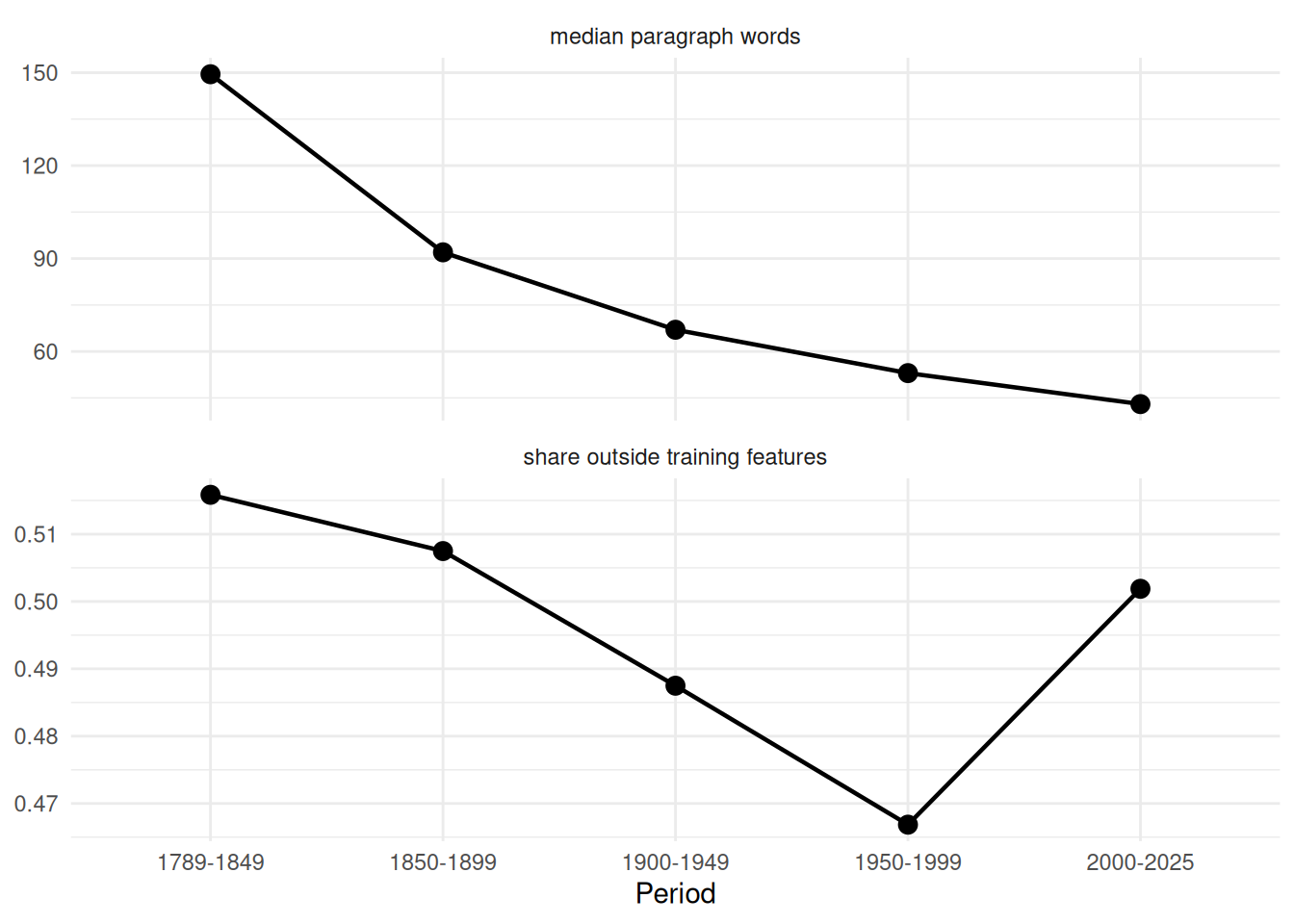
The length pattern is much stronger than the absent-token pattern here. In a live system, either could trigger review. Neither says the model is wrong by itself. It says the input no longer looks the same in a way a person should inspect.
Watch labels as well as words
Concept drift means the relationship between inputs and labels changes over time. Text changes when writers choose new words. Labels can change too.
The party column in this corpus spans the full address range. A label such as Democratic appears across many decades. That span is not evidence that one fixed paragraph model can predict party across the collection. The evaluation result for this recipe and penalty is a measurement warning, not a political finding.
party_range <- paragraphs |>
  summarise(
    first_year = min(year),
    last_year = max(year),
    years_spanned = last_year - first_year,
    parties = n_distinct(party),
    .groups = "drop"
  )

democratic_range <- paragraphs |>
  filter(party == "Democratic") |>
  summarise(
    first_year = min(year),
    last_year = max(year),
    paragraphs = n(),
    speeches = n_distinct(speech_id),
    .groups = "drop"
  )

party_rows <- paragraphs |>
filter(party %in% c("Democratic", "Republican"))| Label scope | First year | Last year | Paragraphs |
|---|---|---|---|
| all party labels | 1789 | 2025 | 1377 |
| Democratic | 1829 | 2021 | 471 |
Monitoring can see the input distribution moving. With checked labels, it can see a score fall. It cannot see confident errors on questions nobody checks. That blind spot is why monitoring needs sampled review, not only dashboards.
What to remember
- Monitoring starts after a model is packaged or put into routine use.
- Slice scores can show where performance changes.
- A slice score is not the same as a new held-out evaluation.
- Concept drift can affect words, labels, or the relationship between them.
- Monitoring cannot find errors in rows that no one checks.
A green dashboard is a prompt to keep looking, not a permanent certificate.