Drawing a knowledge graph

Use IDs, arrows, labels, and tables before reading a layout

information visualization
knowledge graph visualization
networks
Learn how to draw a small knowledge graph in R while keeping identifiers, edge labels, layout limits, and text alternatives visible.

Chloe has a tidy table of Riverton facts, but the table is hard to scan when she wants to follow a path. Which organisation offers the credential? Which deadline values did the knowledge base keep for review? Which place label might cause trouble if IDs were ignored?

Knowledge graph visualization draws entities as nodes and typed relations as edges. In this lesson, the edges are directed and labelled because the relation itself is part of the data.

A drawing can help Chloe see a path. It can also mislead her if she treats the layout as a measurement. The table of edges remains the source of the graph.

Note

The Riverton entities and facts in this lesson are fictional teaching records rebuilt from the earlier knowledge base example.

TipWhat you will learn

By the end of this lesson, you will be able to:

  • key graph nodes by entity ID instead of display label;
  • show how label-keyed data wrongly merges two Riverton places;
  • draw directed, labelled edges with igraph and ggplot2;
  • explain why layout coordinates can change and are not data;
  • give a captioned edge table as the text alternative; and
  • compare a co-word network with a typed knowledge graph.

Rebuild the graph facts by ID

The graph starts with the populated fact edges named in the knowledge-base lesson. The two Riverton places have different IDs. That difference is the first thing the drawing must preserve.

library(dplyr)
library(tibble)
library(tidyr)
library(purrr)
library(stringr)
library(readr)
library(igraph)
library(ggplot2)
library(tidytext)
library(knitr)

source("R/inaugural-corpus.R")

nodes <- tribble(
  ~node_id, ~label, ~node_type,
  "ORG-0002", "Riverton Skills Centre", "organisation",
  "ORG-0003", "Marrow County Transit", "organisation",
  "LOC-0001", "Riverton", "place",
  "LOC-0002", "Riverton", "place",
  "LOC-0003", "Bellhaven", "place",
  "CRD-0002", "Data Support Certificate", "credential",
  "VALUE-October 15", "October 15", "date literal",
  "VALUE-November 1", "November 1", "date literal"
)

edges <- tribble(
  ~from, ~to, ~relation, ~object_value, ~document_ids, ~source,
  "ORG-0002", "CRD-0002", "offers", "CRD-0002", "A001; A002", "populated fact",
  "ORG-0002", "VALUE-October 15", "application_deadline", "October 15", "A003", "populated fact",
  "ORG-0002", "VALUE-November 1", "application_deadline", "November 1", "A004", "populated fact"
)

edge_list <- edges |>
  left_join(
    nodes |> select(from = node_id, from_label = label, from_type = node_type),
    by = "from"
  ) |>
  left_join(
    nodes |> select(to = node_id, to_label = label, to_type = node_type),
    by = "to"
  ) |>
  transmute(
    from_id = from,
    from_label,
    from_type,
    relation = str_replace_all(relation, "_", " "),
    object_value,
    document_ids,
    to_id = to,
    to_label,
    to_type,
    source
  )

knitr::kable(
  edge_list,
  col.names = c(
    "From ID", "From label", "From type", "Relation",
    "Object value", "Document IDs", "To ID", "To label", "To type", "Source"
  ),
  caption = "Every edge drawn in the Riverton knowledge graph",
  row.names = FALSE
)
Every edge drawn in the Riverton knowledge graph
From ID From label From type Relation Object value Document IDs To ID To label To type Source
ORG-0002 Riverton Skills Centre organisation offers CRD-0002 A001; A002 CRD-0002 Data Support Certificate credential populated fact
ORG-0002 Riverton Skills Centre organisation application deadline October 15 A003 VALUE-October 15 October 15 date literal populated fact
ORG-0002 Riverton Skills Centre organisation application deadline November 1 A004 VALUE-November 1 November 1 date literal populated fact

The table is the long description of the graph. It lists every drawn edge with IDs and labels, so the relation can be checked without seeing the picture. The two deadline values are both kept because the knowledge base flagged them as a dated conflict rather than choosing one automatically; no year is supplied in these graph labels because the announcements say only October 15 and November 1.

Show the label-keyed mistake

If the graph used labels as node keys, both Riverton records would collapse into one node. That would merge two different places, so any later fact about one Riverton would appear to belong to the other.

id_graph <- igraph::graph_from_data_frame(
  d = edges,
  directed = TRUE,
  vertices = nodes |> select(name = node_id, label, node_type)
)

label_edges <- edges |>
  left_join(nodes |> select(from = node_id, from_label = label), by = "from") |>
  left_join(nodes |> select(to = node_id, to_label = label), by = "to") |>
  transmute(from = from_label, to = to_label, relation)

label_nodes <- nodes |>
  distinct(name = label, node_type)

label_keyed_graph <- igraph::graph_from_data_frame(
  d = label_edges,
  directed = TRUE,
  vertices = label_nodes
)

merge_check <- tibble(
  key_used = c("entity ID", "display label"),
  vertices = c(igraph::vcount(id_graph), igraph::vcount(label_keyed_graph)),
  riverton_vertices = c(
    sum(igraph::V(id_graph)$label == "Riverton"),
    sum(igraph::V(label_keyed_graph)$name == "Riverton")
  )
)

knitr::kable(
  merge_check,
  col.names = c("Key used", "Vertices", "Vertices displayed as Riverton"),
  caption = "Using labels as keys wrongly merges the two Riverton places",
  row.names = FALSE
)
Using labels as keys wrongly merges the two Riverton places
Key used Vertices Vertices displayed as Riverton
entity ID 8 2
display label 7 1

The ID-keyed graph has eight vertices. The label-keyed graph has seven because the two places named Riverton have been merged.

name_clash <- nodes |>
  count(label, name = "ids_with_label") |>
  filter(ids_with_label > 1L) |>
  left_join(
    nodes |>
      group_by(label) |>
      summarise(
        entity_ids = paste(node_id, collapse = "; "),
        entity_types = paste(node_type, collapse = "; "),
        .groups = "drop"
      ),
    by = "label"
  )

knitr::kable(
  name_clash,
  col.names = c("Shared label", "IDs with label", "Entity IDs", "Entity types"),
  caption = "The name clash is a label problem, not a factual graph edge",
  row.names = FALSE
)
The name clash is a label problem, not a factual graph edge
Shared label IDs with label Entity IDs Entity types
Riverton 2 LOC-0001; LOC-0002 place; place
unconnected_nodes <- nodes |>
  filter(!node_id %in% unique(c(edges$from, edges$to))) |>
  select(node_id, label, node_type)

The figure draws 4 nodes that have no populated fact yet. It places them in its bottom row, and the table below names them.

knitr::kable(
  unconnected_nodes,
  col.names = c("Node ID", "Label", "Type"),
  caption = "Nodes drawn without a populated-fact edge",
  row.names = FALSE
)
Nodes drawn without a populated-fact edge
Node ID Label Type
ORG-0003 Marrow County Transit organisation
LOC-0001 Riverton place
LOC-0002 Riverton place
LOC-0003 Bellhaven place

Place nodes by hand and draw arrows

The main figure uses fixed deterministic coordinates chosen so the labels are readable. That keeps the drawing stable while Chloe reads the arrows and labels. The bottom row holds the nodes with no populated fact. Apart from that row, up, down, left, right, rotation, and mirror image do not carry data. Count links in the table if you need a number. Viewers tend to read a centrally drawn node as more prominent, so the drawing should not be used as an importance score.

layout_from_matrix <- function(graph, coordinates) {
  tibble(
    node_id = igraph::V(graph)$name,
    x = coordinates[, 1],
    y = coordinates[, 2]
  ) |>
    left_join(nodes, by = "node_id")
}

layout_fixed <- tribble(
  ~node_id, ~x, ~y,
  "ORG-0002", 0.0, 0.0,
  "CRD-0002", -2.2, 1.5,
  "VALUE-October 15", 2.2, 1.5,
  "VALUE-November 1", 2.2, -1.1,
  "LOC-0001", -3.0, -3.6,
  "LOC-0002", -1.0, -3.6,
  "ORG-0003", 1.0, -3.6,
  "LOC-0003", 3.0, -3.6
) |>
  left_join(nodes, by = "node_id")

edge_label_positions <- tribble(
  ~from, ~to, ~label_x, ~label_y,
  "ORG-0002", "CRD-0002", -1.25, 0.95,
  "ORG-0002", "VALUE-October 15", 1.30, 0.95,
  "ORG-0002", "VALUE-November 1", 1.35, -0.55
)

shorten_segments <- function(edge_positions, amount = 0.20) {
  edge_positions |>
    mutate(
      x_start = x_from + amount * (x_to - x_from),
      y_start = y_from + amount * (y_to - y_from),
      x_end = x_from + (1 - amount) * (x_to - x_from),
      y_end = y_from + (1 - amount) * (y_to - y_from),
      x_mid = (x_start + x_end) / 2,
      y_mid = (y_start + y_end) / 2
    )
}

edge_positions <- edges |>
  left_join(
    layout_fixed |> select(from = node_id, x_from = x, y_from = y),
    by = "from"
  ) |>
  left_join(
    layout_fixed |> select(to = node_id, x_to = x, y_to = y),
    by = "to"
  ) |>
  left_join(edge_label_positions, by = c("from", "to")) |>
  shorten_segments() |>
  mutate(relation_label = str_replace_all(relation, "_", " "))

node_positions <- layout_fixed |>
  mutate(display_label = paste0(label, "\n", node_id))

graph_plot <- ggplot() +
  geom_segment(
    data = edge_positions,
    aes(x = x_start, y = y_start, xend = x_end, yend = y_end),
    arrow = grid::arrow(type = "closed", length = grid::unit(0.12, "inches")),
    linewidth = 0.4,
    lineend = "round"
  ) +
  geom_label(
    data = edge_positions,
    aes(x = label_x, y = label_y, label = relation_label),
    fill = "white",
    linewidth = 0.15,
    size = 2.8
  ) +
  geom_label(
    data = node_positions,
    aes(x = x, y = y, label = display_label),
    fill = "white",
    linewidth = 0.25,
    size = 3
  ) +
  coord_equal(clip = "off") +
  expand_limits(x = c(-3.7, 3.7), y = c(-4.1, 2.2)) +
  theme_void() +
  theme(plot.margin = margin(15, 15, 15, 15))

graph_plot
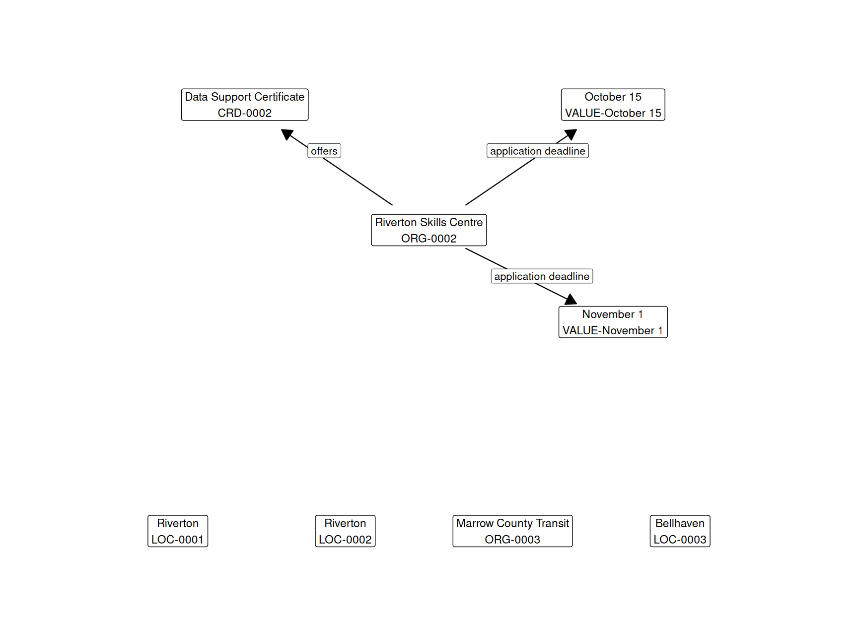
A node-link diagram of 8 nodes, each labelled with a name and an ID, and 3 directed relation edges. The exact edges are listed in the edge table above.
Figure 1: ID-keyed Riverton knowledge graph with directed, labelled edges.

The edge labels are text, not color. The arrowheads show direction, while the caption and table make the same information available outside the image.

Check seed dependence without reading coordinates

Force-directed layouts are useful for many graphs, but their coordinates depend on random starting positions. A layout cannot change the graph’s edges or degrees; it only assigns positions. The check below runs two seeded Fruchterman-Reingold layouts and compares only their coordinates.

layout_for_seed <- function(graph, seed) {
  set.seed(seed)
  layout_from_matrix(
    graph,
    igraph::layout_with_fr(graph, weights = NA)
  )
}

layout_seed_17 <- layout_for_seed(id_graph, 17L)
layout_seed_29 <- layout_for_seed(id_graph, 29L)

seed_comparison <- tibble(
  check = "coordinates identical",
  result = identical(
    layout_seed_17 |> arrange(node_id) |> select(x, y),
    layout_seed_29 |> arrange(node_id) |> select(x, y)
  )
)

knitr::kable(
  seed_comparison,
  col.names = c("Layout check", "Result"),
  caption = "Two force-directed layout seeds produce different coordinates",
  row.names = FALSE
)
Two force-directed layout seeds produce different coordinates
Layout check Result
coordinates identical FALSE

Use the main layout to follow labelled arrows. The seeded force-layout check is there only to show why coordinates should not be treated as facts.

Build a co-word network for comparison

A co-word network is a different graph. Its nodes are words. Its edges are undirected and based on how often two words appear in the same unit. Here the unit is an inaugural paragraph. The word rule keeps alphabetic tokens of four or more letters, lowercases them in English, removes tidytext stop words, and uses paragraph presence rather than raw repeated counts.

paragraphs <- inaugural_paragraphs()

paragraph_words <- paragraphs |>
  transmute(paragraph_id, paragraph) |>
  tidytext::unnest_tokens(word, paragraph, token = "regex", pattern = "[^A-Za-z]+") |>
  mutate(word = str_to_lower(word, locale = "en")) |>
  filter(nchar(word) >= 4L) |>
  anti_join(tidytext::stop_words, by = "word") |>
  distinct(paragraph_id, word)

top_words <- paragraph_words |>
  count(word, name = "paragraphs_with_word", sort = TRUE) |>
  slice_head(n = 10)

top_word_presence <- paragraph_words |>
  semi_join(top_words, by = "word")

word_pairs <- top_word_presence |>
  inner_join(top_word_presence, by = "paragraph_id", relationship = "many-to-many") |>
  filter(word.x < word.y) |>
  count(word.x, word.y, name = "observed") |>
  left_join(top_words, by = c("word.x" = "word")) |>
  rename(first_paragraphs = paragraphs_with_word) |>
  left_join(top_words, by = c("word.y" = "word")) |>
  rename(second_paragraphs = paragraphs_with_word) |>
  mutate(
    total_paragraphs = n_distinct(paragraphs$paragraph_id),
    expected = first_paragraphs * second_paragraphs / total_paragraphs,
    observed_expected_ratio = observed / expected
  )

ratio_threshold <- 1.80
coword_edges <- word_pairs |>
  filter(observed_expected_ratio >= ratio_threshold) |>
  arrange(desc(observed_expected_ratio), word.x, word.y)

kept_pair_count <- nrow(coword_edges)
dropped_pair_count <- nrow(word_pairs) - kept_pair_count
undrawn_words <- setdiff(top_words$word, unique(c(coword_edges$word.x, coword_edges$word.y)))

knitr::kable(
  top_words,
  col.names = c("Word", "Paragraphs with word"),
  caption = "Top ten content words after the paragraph-level word rule",
  row.names = FALSE
)
Top ten content words after the paragraph-level word rule
Word Paragraphs with word
people 409
government 358
nation 268
country 259
world 251
citizens 196
time 189
peace 172
power 169
america 167
knitr::kable(
  coword_edges |>
    mutate(
      expected = round(expected, 1),
      observed_expected_ratio = round(observed_expected_ratio, 2)
    ),
  col.names = c(
    "First word", "Second word", "Observed paragraphs",
    "First word paragraphs", "Second word paragraphs",
    "Total paragraphs", "Expected under independence",
    "Observed / expected"
  ),
  caption = "Co-word edges kept by the observed-versus-expected threshold",
  row.names = FALSE
)
Co-word edges kept by the observed-versus-expected threshold
First word Second word Observed paragraphs First word paragraphs Second word paragraphs Total paragraphs Expected under independence Observed / expected
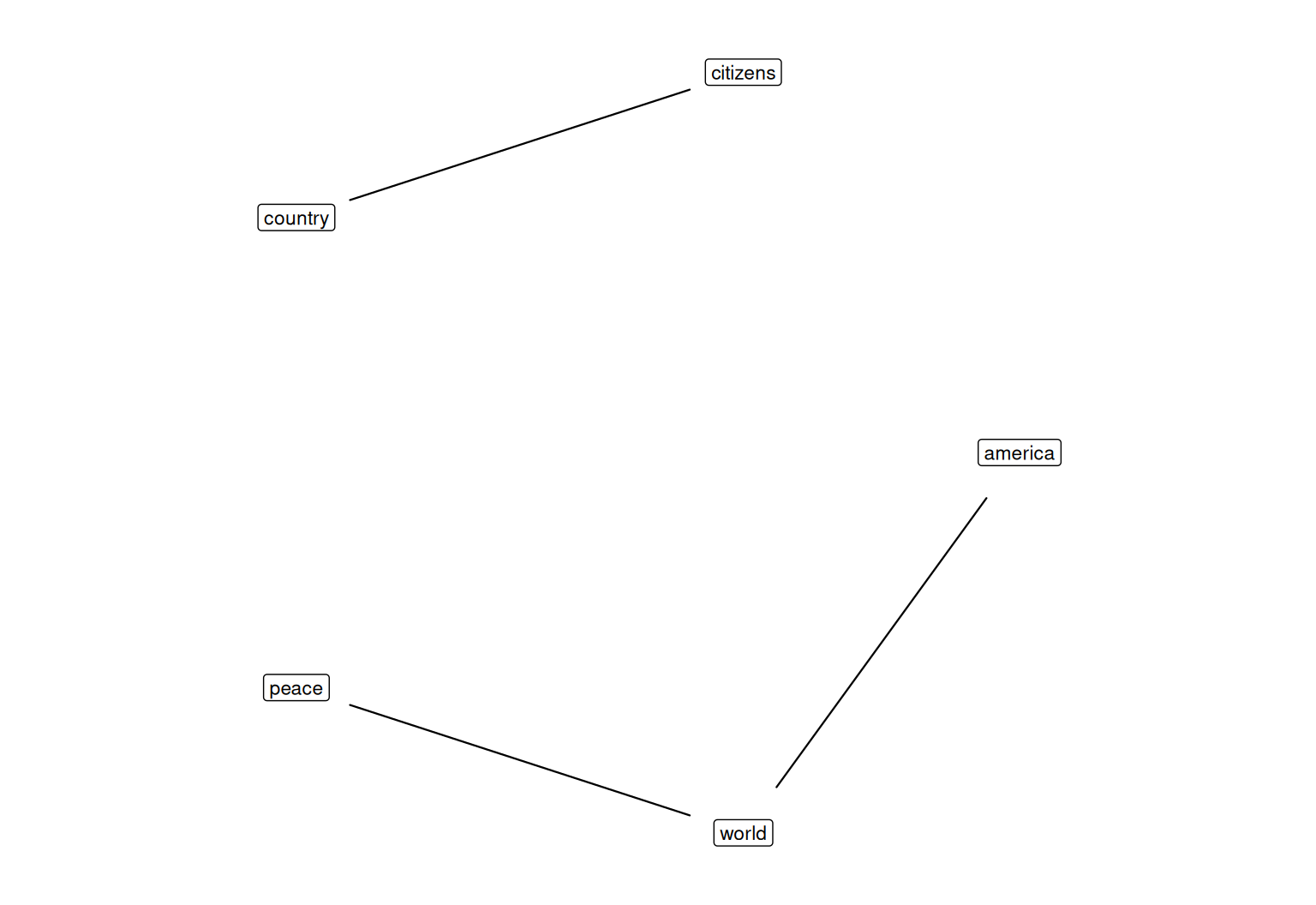
peace world 68 172 251 1377 31.4 2.17
america world 58 167 251 1377 30.4 1.91
citizens country 70 196 259 1377 36.9 1.90
threshold_summary <- tibble(
  threshold = ratio_threshold,
  kept_pairs = kept_pair_count,
  dropped_pairs = dropped_pair_count,
  undrawn_top_words = paste(undrawn_words, collapse = ", ")
)

knitr::kable(
  threshold_summary,
  col.names = c("Observed / expected threshold", "Kept pairs", "Dropped pairs", "Top words not drawn"),
  caption = "The author's co-word threshold decides which word pairs are drawn",
  row.names = FALSE
)
The author’s co-word threshold decides which word pairs are drawn
Observed / expected threshold Kept pairs Dropped pairs Top words not drawn
1.8 3 42 people, government, nation, time, power

Raw co-occurrence among these ten frequent words is a complete graph: all 45 pairs appear in at least one paragraph. The threshold is the author’s choice for this lesson. It keeps 3 pairs and drops 42 pairs by requiring the observed count to be at least 1.8 times the independence expectation count(word A) * count(word B) / paragraphs. The undrawn top-ten words are people, government, nation, time, power.

Draw the co-word graph

The co-word graph uses the same drawing machinery, but its edges are not typed facts. They are paragraph-level co-occurrences that passed the threshold.

coword_nodes <- tibble(
  node_id = sort(unique(c(coword_edges$word.x, coword_edges$word.y))),
  label = node_id
)

coword_graph <- igraph::graph_from_data_frame(
  d = coword_edges |>
    transmute(from = word.x, to = word.y, relation = "co-occurs"),
  directed = FALSE,
  vertices = coword_nodes |> select(name = node_id, label)
)

coword_layout_matrix <- igraph::layout_in_circle(coword_graph)
coword_layout <- tibble(
  node_id = igraph::V(coword_graph)$name,
  x = coword_layout_matrix[, 1],
  y = coword_layout_matrix[, 2]
) |>
  left_join(coword_nodes, by = "node_id")

coword_positions <- coword_edges |>
  transmute(from = word.x, to = word.y, relation = "co-occurs") |>
  left_join(
    coword_layout |> select(from = node_id, x_from = x, y_from = y),
    by = "from"
  ) |>
  left_join(
    coword_layout |> select(to = node_id, x_to = x, y_to = y),
    by = "to"
  ) |>
  shorten_segments(amount = 0.12)

coword_plot <- ggplot() +
  geom_segment(
    data = coword_positions,
    aes(x = x_start, y = y_start, xend = x_end, yend = y_end),
    linewidth = 0.4,
    lineend = "round"
  ) +
  geom_label(
    data = coword_layout,
    aes(x = x, y = y, label = label),
    fill = "white",
    linewidth = 0.25,
    size = 3
  ) +
  coord_equal(clip = "off") +
  theme_void() +
  theme(plot.margin = margin(15, 15, 15, 15))

coword_plot
An undirected co-word diagram whose nodes are content words and whose edges are thresholded paragraph co-occurrences. The kept edges and counts are listed in the table 'Co-word edges kept by the observed-versus-expected threshold'.
Figure 2: Co-word network for the three top-word pairs that passed the observed-versus-expected threshold.

Unlike the Riverton knowledge graph, this co-word network has no entity IDs, no relation types, and no direction. It can show which word pairs survived a preprocessing and threshold decision. It cannot say that the words mean the same thing or that one caused the other to appear.

What to remember

  • Use stable IDs as node keys; labels can collide.
  • The two Riverton places merge if labels are treated as IDs.
  • A force-directed layout is a computed drawing, not a measurement.
  • Arrowheads and relation labels carry the graph meaning.
  • The edge-list table is part of the graph’s text alternative.
  • Co-word edges are thresholded co-occurrences, not typed knowledge-base facts.

Start with the edge table, then use the drawing only as a guide to the paths it lists.

Sources