suppressPackageStartupMessages({
  library(readr)
  library(dplyr)
  library(tidyr)
  library(tibble)
  library(stringr)
  library(ggplot2)
  library(rsample)
  library(recipes)
  library(textrecipes)
  library(parsnip)
  library(workflows)
  library(yardstick)
  library(broom)
  library(glmnet)
})

study <- read_csv(
  "data/inaugural/split-study.csv",
  na = c("", "NA"),
  col_types = cols(
    task = col_character(),
    split_scheme = col_character(),
    replicate = col_integer(),
    accuracy = col_double(),
    bal_accuracy = col_double(),
    train_majority_accuracy = col_double(),
    test_majority_rate = col_double(),
    length_rule_accuracy = col_double(),
    test_rows = col_integer(),
    test_speeches = col_integer()
  )
)

baselines <- read_csv(
  "data/inaugural/baselines.csv",
  na = character(),
  col_types = cols(
    task = col_character(),
    outcome = col_character(),
    rows = col_integer(),
    speeches = col_integer(),
    people = col_integer(),
    largest_class = col_character(),
    baseline_accuracy = col_double()
  )
)

split_levels <- c("paragraph", "speech", "president")
task_levels <- c("era", "era_party_rows", "party")

task_labels <- c(
  era = "era",
  era_party_rows = "era on party rows",
  party = "party"
)

split_summary <- study |>
  mutate(
    task = factor(task, levels = task_levels),
    split_scheme = factor(split_scheme, levels = split_levels)
  ) |>
  group_by(task, split_scheme) |>
  summarise(
    replicates = n(),
    mean_accuracy = mean(accuracy),
    mean_bal_accuracy = mean(bal_accuracy, na.rm = TRUE),
    bal_accuracy_missing = sum(is.na(bal_accuracy)),
    mean_train_majority = mean(train_majority_accuracy),
    mean_test_majority = mean(test_majority_rate),
    mean_length_rule = mean(length_rule_accuracy),
    low_accuracy = min(accuracy),
    high_accuracy = max(accuracy),
    low_train_majority = min(train_majority_accuracy),
    high_train_majority = max(train_majority_accuracy),
    low_length_rule = min(length_rule_accuracy),
    high_length_rule = max(length_rule_accuracy),
    mean_test_speeches = mean(test_speeches),
    .groups = "drop"
  ) |>
  arrange(task, split_scheme)

baseline_display <- baselines |>
  mutate(task = factor(task, levels = task_levels)) |>
  arrange(task) |>
  transmute(
    task = recode(as.character(task), !!!task_labels),
    rows,
    speeches,
    people,
    largest_class,
    baseline_accuracy
)Evaluating models
Read a score only after asking what it was compared with
model development
evaluation
text classification
Learn why model evaluation needs a baseline, repeated splits, and a split scheme that matches the claim.
A program manager sees one number on a slide: 61 percent accurate. It sounds better than guessing, so the room starts to relax.
Then she asks what the model would have scored if it had always chosen the larger class. The answer changes the meeting. The score was not evidence of a working model after all.
This lesson reads a committed split study for three related text models. The era model is useful against cheap alternatives. The party model, with these features and this fixed penalty, does not learn a reliable party signal.
TipWhat you will learn
This lesson shows how to:
- separate candidate selection, final testing, and robustness checks;
- compare every score with a deployable largest-class baseline;
- read the spread across repeated train/test splits;
- explain what paragraph, speech, and person splits measure;
- use a confusion matrix and balanced accuracy; and
- say when a specific model did not learn the target.
Start with the baseline
A baseline is the simple rule a model has to beat. The largest-class baseline always predicts the most common label in training data. It is crude, which is exactly why it is a useful check. If a model cannot beat that rule, its score should not be sold as success.
| Task | Rows | Speeches | People | Largest class | Corpus baseline |
|---|---|---|---|---|---|
| era | 1377 | 60 | 40 | 1900 or later | 0.6478 |
| era on party rows | 1197 | 47 | 31 | 1900 or later | 0.7452 |
| party | 1197 | 47 | 31 | Republican | 0.6065 |
The era task has 1377 rows, 60 speeches, and 40 people. The party model can train only on rows with a Democratic or Republican label, so it uses 1197 rows from 47 speeches by 31 people. The remaining rows come from other party labels. Each task also selects its own 500 tokens from its own training data.
Selection, testing, and robustness do different jobs
Lesson 43 compared candidate settings with five grouped folds made only from the training speeches. It then used the 14 untouched test speeches once, after the candidate and penalty were fixed. That is the final test for that modeling decision inside this worked example. A new corpus would be needed to test whether the result transfers to another collection.
The repeated study below asks a different question. It redraws the split 10 times to show how scores move when different speeches land on each side. These repeated holdouts are a robustness check, not 10 new untouched test sets, and they were not used to choose the candidate in lesson 43.
Accuracy is the share of rows with the right label. When classes are uneven, a model can get many rows right by favoring the larger class. A confusion matrix shows which labels were confused, and balanced accuracy averages the accuracy within each class so the smaller class still counts.
Repeated splits change the answer
The study runs 10 replicates for each task and split scheme. A replicate is a fresh split made by the same rule. The mean tells the center of the results, and the low and high values show how much the score moved across the 10 runs. Unlike five-fold cross-validation, a repeated holdout does not guarantee that every speech takes one turn in assessment. Its purpose here is sensitivity to the split, not model selection.
score_table <- split_summary |>
  transmute(
    task = recode(as.character(task), !!!task_labels),
    split_scheme = as.character(split_scheme),
    mean_accuracy = round(mean_accuracy, 4),
    mean_bal_accuracy = round(mean_bal_accuracy, 4),
    train_majority_accuracy = round(mean_train_majority, 4),
    test_majority_rate = round(mean_test_majority, 4),
    length_rule_accuracy = round(mean_length_rule, 4),
    low_accuracy = round(low_accuracy, 4),
    high_accuracy = round(high_accuracy, 4),
    missing_bal_accuracy = bal_accuracy_missing
  )

get_summary <- function(task_name, scheme_name) {
  split_summary |>
    filter(task == task_name, split_scheme == scheme_name)
}

era_speech <- get_summary("era", "speech")
era_president <- get_summary("era", "president")
era_party_speech <- get_summary("era_party_rows", "speech")
era_party_president <- get_summary("era_party_rows", "president")
party_paragraph <- get_summary("party", "paragraph")
party_speech <- get_summary("party", "speech")
party_president <- get_summary("party", "president")

na_replicate <- study |>
  filter(task == "era_party_rows", split_scheme == "president", is.na(bal_accuracy))

era_speech_range_width <- era_speech$high_accuracy - era_speech$low_accuracy

era_speech_length_gap <- era_speech$mean_accuracy - era_speech$mean_length_rule

era_party_speech_gap <- era_party_speech$mean_accuracy - era_party_speech$mean_train_majority

paired_comparisons <- bind_rows(
  study |>
    filter(task == "era", split_scheme == "speech") |>
    summarise(
      comparison = "era, all rows",
      model_wins = sum(accuracy > train_majority_accuracy),
      ties = sum(accuracy == train_majority_accuracy),
      model_losses = sum(accuracy < train_majority_accuracy)
    ),
  study |>
    filter(task == "era_party_rows", split_scheme == "speech") |>
    summarise(
      comparison = "era, party rows",
      model_wins = sum(accuracy > train_majority_accuracy),
      ties = sum(accuracy == train_majority_accuracy),
      model_losses = sum(accuracy < train_majority_accuracy)
    ),
  study |>
    filter(task == "party", split_scheme == "paragraph") |>
    summarise(
      comparison = "party, paragraph split",
      model_wins = sum(accuracy > train_majority_accuracy),
      ties = sum(accuracy == train_majority_accuracy),
      model_losses = sum(accuracy < train_majority_accuracy)
    )
)

party_president_bal_range <- range(
  study$bal_accuracy[
    study$task == "party" &
      study$split_scheme == "president"
  ]
)| Task | Split | Model accuracy | Balanced accuracy | Training-majority rule | Test-majority rate | Length rule | Model low | Model high | Missing balanced accuracy |
|---|---|---|---|---|---|---|---|---|---|
| era | paragraph | 0.8661 | 0.8617 | 0.6464 | 0.6464 | 0.6652 | 0.8406 | 0.9043 | 0 |
| era | speech | 0.8457 | 0.8516 | 0.6282 | 0.6712 | 0.6827 | 0.7970 | 0.9039 | 0 |
| era | president | 0.8354 | 0.8206 | 0.6185 | 0.6266 | 0.7184 | 0.7543 | 0.8782 | 0 |
| era on party rows | paragraph | 0.8473 | 0.8059 | 0.7433 | 0.7433 | 0.6057 | 0.8233 | 0.8833 | 0 |
| era on party rows | speech | 0.8240 | 0.7641 | 0.8086 | 0.8086 | 0.5931 | 0.7362 | 0.8810 | 0 |
| era on party rows | president | 0.8521 | 0.8143 | 0.8284 | 0.8284 | 0.6871 | 0.8094 | 0.9033 | 1 |
| party | paragraph | 0.6060 | 0.5887 | 0.6067 | 0.6067 | 0.5077 | 0.5700 | 0.6400 | 0 |
| party | speech | 0.5514 | 0.5408 | 0.6563 | 0.6806 | 0.4148 | 0.4561 | 0.6055 | 0 |
| party | president | 0.4997 | 0.5090 | 0.4914 | 0.6173 | 0.4308 | 0.4158 | 0.5631 | 0 |
| Comparison | Model wins | Ties | Model losses |
|---|---|---|---|
| era, all rows | 10 | 0 | 0 |
| era, party rows | 6 | 0 | 4 |
| party, paragraph split | 3 | 1 | 6 |
The speech split is the main era test. The model averages 0.8457, while the deployable majority rule averages 0.6282 and the paragraph-length rule averages 0.6827. The model’s lowest speech-split replicate is 0.797, which is still higher than the best mean reached by either cheap rule. Across the 10 speech replicates, the model ranges from 0.797 to 0.9039. The deployable rule ranges from 0.3576 to 0.8318, and the length rule ranges from 0.5255 to 0.8498.
A score is meaningful only against the best cheap alternative you bothered to try. Here the length rule matters because paragraph length is confounded with era. The model still beats that one-number rule by about 16.3 points at the speech split, so the text features are doing real work.
Show the plotting code
source("R/lesson-figures.R")

plot_data <- study |>
  filter(task %in% c("era", "party")) |>
  mutate(
    task = recode(task, !!!task_labels),
    split_scheme = factor(split_scheme, levels = split_levels)
  ) |>
  select(task, split_scheme, replicate, accuracy, train_majority_accuracy, length_rule_accuracy) |>
  pivot_longer(
    cols = c(accuracy, train_majority_accuracy, length_rule_accuracy),
    names_to = "measure",
    values_to = "score"
  ) |>
  mutate(
    measure = recode(
      measure,
      accuracy = "model",
      train_majority_accuracy = "training-majority rule",
      length_rule_accuracy = "paragraph-length rule"
    )
  )

mean_scores <- plot_data |>
  summarise(score = mean(score), .by = c(task, split_scheme, measure))

measure_colours <- c(
  "model" = lesson_colours[["accent"]],
  "training-majority rule" = lesson_colours[["contrast"]],
  "paragraph-length rule" = lesson_colours[["support"]]
)
measure_label_colours <- c(
  "model" = lesson_text_colours[["accent"]],
  "training-majority rule" = lesson_text_colours[["contrast"]],
  "paragraph-length rule" = lesson_text_colours[["support"]]
)

# The y scale is left to the data. Fixing the lower bound at 0.3 would drop the
# two replicates where the training-majority rule scores 0.27, and those
# are exactly the cases worth seeing: the rule collapses when the class that was
# largest in training is the smaller one in test.
ggplot(plot_data, aes(x = split_scheme, y = score, colour = measure)) +
  geom_point(
    alpha = 0.35,
    size = 1.5,
    position = position_jitter(width = 0.08, height = 0, seed = 4401)
  ) +
  geom_line(
    data = mean_scores,
    aes(group = measure, linetype = measure),
    linewidth = 0.9
  ) +
  geom_point(data = mean_scores, size = 2.6) +
  ggrepel::geom_text_repel(
    data = mean_scores |>
      filter(split_scheme == last(split_levels)),
    aes(label = measure, colour = I(measure_label_colours[measure])),
    direction = "y",
    hjust = 0,
    nudge_x = 0.3,
    segment.colour = NA,
    family = lesson_font,
    size = 3.4,
    seed = 4402
  ) +
  facet_wrap(vars(task)) +
  scale_colour_manual(values = measure_colours, guide = "none") +
  scale_linetype_manual(
    values = c(
      "model" = "solid",
      "training-majority rule" = "22",
      "paragraph-length rule" = "42"
    ),
    guide = "none"
  ) +
  scale_x_discrete(expand = expansion(add = c(0.3, 2.1))) +
  scale_y_continuous(labels = scales::label_number(accuracy = 0.01)) +
  labs(
    title = "The model beats both cheap rules for era but not clearly for party",
    subtitle = "Accuracy in 10 replicates per split scheme; lines join the replicate means",
    x = "Split scheme",
    y = "Accuracy"
  ) +
  theme_lesson(grid = "y")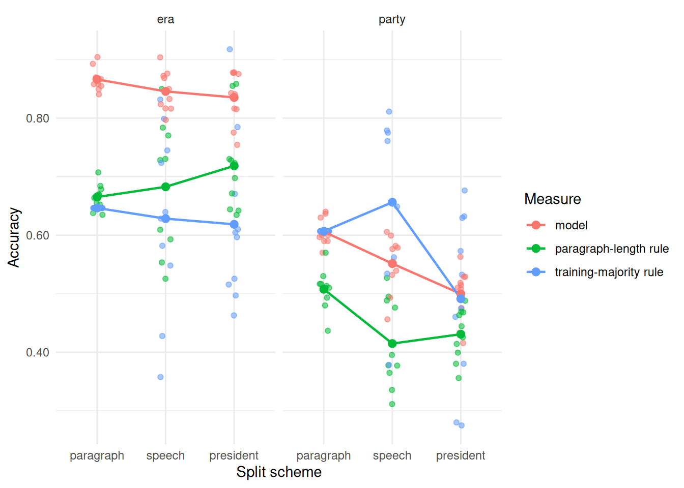
The party model does not beat its deployable majority rule on average at the paragraph split: 0.606 for the model against 0.6067 for the rule. Across the 10 paired replicates, the model wins 3, ties 1, and loses 6. At the speech split, the model averages 0.5514 against 0.6563. Under the person split, accuracy is 0.4997 and mean balanced accuracy is 0.509. Its replicate values range from 0.4769 to 0.5595, straddling the theoretical two-class chance value of 0.5. The conclusion is model-level: this penalty, recipe, and row set did not learn party reliably.
The controlled comparison is smaller
The era and party tasks are not a clean pair by default. Party keeps only the Democratic and Republican speeches, which leaves 1197 of the full 1377 paragraphs. The dropped rows are from other party labels, and those rows are concentrated in the earliest speeches with longer paragraphs.
The controlled comparison is era_party_rows, which runs the era label on the same rows as the party model. On the full era corpus, the model beats the deployable rule in all 10 speech-level replicates. On the party-row subset, the model averages 0.824 against 0.8086 for the training-majority rule, but it wins 6 paired replicates and loses 4. The mean gap is only 1.5 points because this subset is much more imbalanced, and its direction is not stable across splits. Era is learnable on the full rows here and party is not learned by this model, but the controlled subset does not support the same strong era conclusion.
For era_party_rows under the person split, replicate 3 has undefined balanced accuracy because the test set has only one class. Its test-majority rate is 1, so the accuracy for that one replicate is not a two-class result. The summary table uses na.rm = TRUE for balanced accuracy and reports the missing count so the case stays visible.
Read the final confusion matrix
Sensitivity is the share of before 1900 paragraphs assigned to that first factor level. Specificity is the share of 1900 or later paragraphs assigned to the second level. Naming the event level matters because reversing the factor levels reverses which class each measure describes.
source("R/inaugural-corpus.R")
paragraphs <- inaugural_paragraphs()

set.seed(4301)
era_split <- group_initial_split(paragraphs, group = speech_id, prop = 0.75)
era_training <- training(era_split)
era_testing <- testing(era_split)

era_recipe <- recipe(era ~ paragraph, data = era_training) |>
  step_tokenize(paragraph) |>
  step_stopwords(paragraph) |>
  step_tokenfilter(paragraph, max_tokens = 500) |>
  step_tfidf(paragraph)

era_model <- logistic_reg(penalty = 0.01, mixture = 0) |>
  set_engine("glmnet")

era_workflow <- workflow() |>
  add_recipe(era_recipe) |>
  add_model(era_model)

set.seed(4302)
era_fitted <- fit(era_workflow, data = era_training)

era_predictions <- predict(era_fitted, era_testing) |>
  bind_cols(era_testing |> select(era))

final_training_majority <- era_training |>
  count(era, sort = TRUE) |>
  slice(1) |>
  pull(era)
final_split_baseline <- mean(era_testing$era == final_training_majority)

confusion <- conf_mat(
  era_predictions,
  truth = era,
  estimate = .pred_class
)
confusion_table <- as.data.frame(confusion$table) |>
  as_tibble()

metric_table <- metric_set(accuracy, bal_accuracy, sens, spec)(
  era_predictions,
  truth = era,
  estimate = .pred_class
) |>
  select(.metric, .estimate) |>
  bind_rows(
    tibble(
      .metric = "training_majority_accuracy",
      .estimate = final_split_baseline
    )
)| Prediction | Reference label | Paragraphs |
|---|---|---|
| before 1900 | before 1900 | 145 |
| 1900 or later | before 1900 | 50 |
| before 1900 | 1900 or later | 10 |
| 1900 or later | 1900 or later | 130 |
| Measure | Value |
|---|---|
| accuracy | 0.8209 |
| bal_accuracy | 0.8361 |
| sens | 0.7436 |
| spec | 0.9286 |
| training_majority_accuracy | 0.4179 |
The model gets 145 early-era paragraphs right and misses 50 of them. It gets 130 later-era paragraphs right and misses 10 of them. Balanced accuracy is 0.8361, which gives both classes equal weight. The model accuracy is 0.8209; the deployable training-majority rule scores 0.4179 on these same rows.
What else could produce this score
Era is a deterministic function of year, and year is constant within a speech. The era study has 60 independent speech units, not 1377 independent paragraphs. The speech split averages about 14.7 speeches per test set. That is why the model range across speech splits is 0.1069, not the tighter range one might expect from hundreds of independent rows. The 10 replicates describe resampling variability inside one corpus; they are not a confidence interval for political speech beyond this collection.
The next lesson prints this model’s largest coefficients. Read them when you get there, because they cut both ways. The terms pushing toward the earlier label are mostly formal-register words, the vocabulary of a certain kind of nineteenth- century public address rather than a certain kind of subject. The terms pushing the other way include words like industrial, economic, international, and federal, which are closer to genuine changes in what the speeches are about. So part of this score is a style detector and part of it is a subject detector, and nothing here separates the two. Nineteenth- and twenty-first-century texts can also differ because of transcription and typesetting conventions, which no measurement on this page would distinguish from either.
This lesson supports the limited claim that era is learnable from this text. It does not show that the model learned what a period was about. A features-only stylometric model, or a subsample matched on paragraph length, would be needed to pull period vocabulary apart from period register.
When a model grades another model
Generated text rarely has one right answer, so many projects now ask a language model to score other outputs. Large comparisons find that model judges agree with people well on some tasks and poorly on others, and that they can favour an answer because of its position in the prompt or its length. A judge is a measuring instrument like the classifier on this page. Before using its scores, compare them with human ratings on a random sample from your own task, swap the order of the answers it compares, and report agreement with a chance-corrected statistic such as Cohen’s kappa. The guide Using a language model in a reproducible analysis shows the same checking pattern for model labels.
What to remember
- A score with no baseline is hard to interpret.
- Candidate selection must finish before the final test set is opened.
- Group splits need same-split baselines, not only corpus-wide baselines.
- One split gives one number; repeated splits show the spread.
- The split scheme decides what the score is measuring.
- This text model learned era well. This model, with this penalty and these features, did not learn party, which is a smaller claim than saying the task is impossible.
- A language model used as a judge needs the same checks against people.
A useful evaluation does not flatter the model. It tells you which answer you are allowed to trust.
Sources
- yardstick metrics reference
- rsample initial splits
- rsample grouped splits
- rsample grouped V-fold cross-validation
- tidymodels tuning
- tidymodels workflows
- Zheng et al. (2023), Judging LLM-as-a-judge with MT-Bench and Chatbot Arena
- Bavaresco et al. (2025), LLMs instead of human judges? A large-scale empirical study across 20 NLP evaluation tasks